心脏疾病数据分析: Wolfram 语言 11 的新功能

心脏疾病数据分析

数据分析是基于从原始数据源提取的信息的提取、演示、建模过程. 本范例展示了用 Wolfram 语言进行数据分析的一个工作流程. 这里使用的数据集来自 UCI Machine Learning Repository，包含了 1,541 名患者的心脏疾病诊断数据.

导入心脏疾病诊断数据，并对其解析使得每行与不同患者相对应，并且每列对应不同属性.

In[1]:=

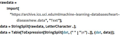
rawdata = 
  Import["https://archive.ics.uci.edu/ml/machine-learning-databases/\
heart-disease/new.data", "Text"];
data = StringSplit[rawdata, LetterCharacter ..];
data = Table[
   ToExpression[StringSplit[dat, (" " | "\n") ..]], {dat, data}];

将相关属性提取至 "labels" 和 "features". "labels" 中存储的值为 0 和 1，分别对应心脏疾病的 presence（存在）和 absence（不存在）.

In[2]:=

labels = Unitize[data[[All, 58]]];
features = 
  data[[All, {3, 4, 9, 10, 12, 16, 19, 32, 38, 40, 41, 44, 51}]];

In[3]:=

Take[labels, 10]

Out[3]=

对于每位患者，特征向量是数字值的列表. 但是，数据并不完整且缺失域储存为 .

In[4]:=

features[[-3]]

Out[4]=

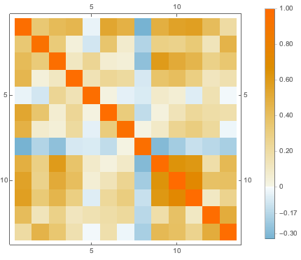
用对应属性中可用数据的平均值来置换缺失的值，然后可视化不同属性的关联.

In[5]:=

features = Transpose[Table[
    N[attribute /. {-9 -> Mean[N[DeleteCases[attribute, -9]]]}]
    , {attribute, Transpose[features]}]];
cormat = Correlation[features];

显示完整的 Wolfram 语言输入

In[6]:=

MatrixPlot[cormat, ImageSize -> Medium, PlotTheme -> "Detailed"]

Out[6]=

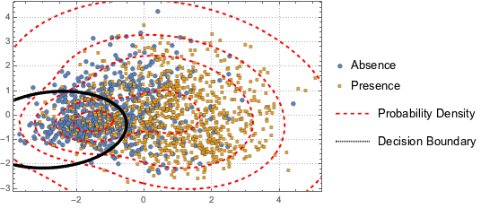
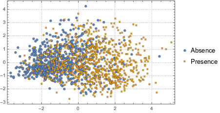
为可视化数据分布, 用 PCA 操作提取前两个分量，然后将投影数据绘在散点图上.

In[7]:=

pcs2 = Take[PrincipalComponents[features, Method -> "Correlation"], 
   All, 2];

显示完整的 Wolfram 语言输入

In[8]:=

splot = With[{ind = Pick[Range[Length[pcs2]], labels, 0]},
  ListPlot[{pcs2[[ind]], Delete[pcs2, Transpose[{ind}]]}, 
   ImageSize -> Medium, PlotTheme -> "Detailed", 
   PlotMarkers -> Automatic, PlotLegends -> {"Absence", "Presence"}]
  ]

Out[8]=

为区分两个分类，用一个二分量高斯混合模型拟合投影数据.

In[9]:=

edist = EstimatedDistribution[pcs2, 
   MixtureDistribution[{p1, 
     p2}, {BinormalDistribution[{m11, m12}, {s11, s12}, r1], 
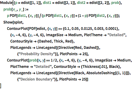
     BinormalDistribution[{m21, m22}, {s21, s22}, r2]}]];

根据混合模型，绘制混合模型的决策边界（黑色曲线）和概率密度等值线（红色曲线）并与散点绘图一同显示. 高斯混合的第一个分量在决策边界中的概率更高.

显示完整的 Wolfram 语言输入

In[10]:=

Module[{p = edist[[1, 1]], dist1 = edist[[2, 1]], 
  dist2 = edist[[2, 2]], prob},
 prob[x_, y_] := 
  p PDF[dist1, {x, 
      y}]/(p PDF[dist1, {x, y}] + (1 - p) PDF[dist2, {x, y}]);
 Show[splot, 
  ContourPlot[
   PDF[edist, {x, y}] == {0.1, 0.05, 0.0125, 0.003, 0.0001}, {x, -4, 
    6}, {y, -4, 6}, ImageSize -> Medium, PlotTheme -> "Detailed", 
   ContourStyle -> {Dashed, Thick, Red}, 
   PlotLegends -> 
    LineLegend[{Directive[Red, Dashed]}, {"Probability Density"}], 
   PlotPoints -> 25], 
  ContourPlot[prob[x, y] == 1/2, {x, -4, 6}, {y, -4, 6}, 
   ImageSize -> Medium, PlotTheme -> "Detailed", 
   ContourStyle -> {Thickness[.01], Black}, 
   PlotLegends -> 
    LineLegend[{Directive[Black, 
       AbsoluteDashing[{1, 1}]]}, {"Decision Boundary"}], 
   PlotPoints -> 25]]
 ]

Out[10]=

Wolfram 语言™

心脏疾病数据分析

相关范例