Solve an Initial Value Problem for the Wave Equation
Specify the wave equation with unit speed of propagation.
In[1]:=
weqn = D[u[x, t], {t, 2}] == D[u[x, t], {x, 2}];Prescribe initial conditions for the equation.
In[2]:=
ic = {u[x, 0] == E^(-x^2), Derivative[0, 1][u][x, 0] == 1};Solve the initial value problem.
In[3]:=
DSolveValue[{weqn, ic}, u[x, t], {x, t}]Out[3]=
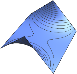
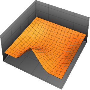
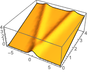
The wave propagates along a pair of characteristic directions.
In[4]:=
DSolveValue[{weqn, ic}, u[x, t], {x, t}];
Plot3D[%, {x, -7, 7}, {t, 0, 4}, Mesh -> None]
Out[4]=
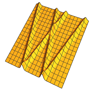
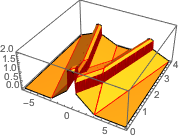
Solve the initial value problem with piecewise data.
In[5]:=
ic = {u[x, 0] == UnitBox[x] + UnitTriangle[x/3],
   Derivative[0, 1][u][x, 0] == 0};
In[6]:=
DSolveValue[ {weqn, ic}, u[x, t], {x, t}]Out[6]=
Discontinuities in the initial data are propagated along the characteristic directions.
In[7]:=
DSolveValue[ {weqn, ic}, u[x, t], {x, t}];
Plot3D[%, {x, -7, 7}, {t, 0, 4}, PlotRange -> All, Mesh -> None,
 ExclusionsStyle -> Red]
Out[7]=
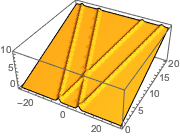
Solve the initial value problem with a sum of exponential functions as initial data.
In[8]:=
ic = {u[x, 0] == E^(-(x - 6)^2) + E^(-(x + 6)^2),
       Derivative[0, 1][u][x, 0] == 1/2};
In[9]:=
sol = DSolveValue[ {weqn, ic}, u[x, t], {x, t}]Out[9]=
Visualize the solution.
In[10]:=
Plot3D[sol, {x, -30, 30}, {t, 0, 20}, PlotRange -> All, Mesh -> None,
 PlotPoints -> 30]
Out[10]=