핵심 알고리즘
정교한 혼합 모델에서의 비모수 분포
두꺼운 꼬리 데이터의 준 모수 모델입니다. 꼬리 부분은 최대 가능도를 통한 코시 분포 추정으로 절단된 것입니다. 모델의 중심 부분은 데이터의 비모수 핵 밀도로 추정된 것입니다.
| In[1]:= | 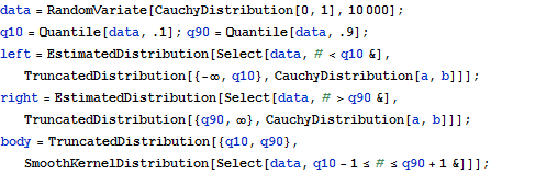 X |
| In[2]:= | X |
| In[3]:= | 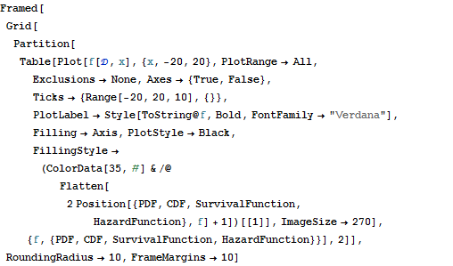 X |
| Out[3]= | 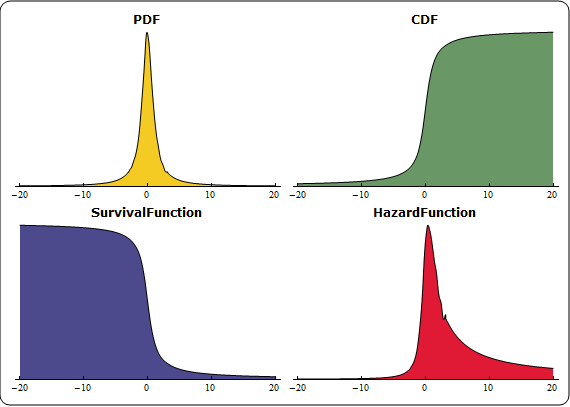 |
| Wolfram Mathematica 8의 신기능: 비모수 분포, 파생 분포, 포뮬라 분포 | ◄ 이전 | 다음 ► |
| In[1]:= | X |
| In[2]:= | X |
| In[3]:= | X |
| Out[3]= | |