Algoritmos de núcleo
Compare funciones de distribución para cópulas estimadas y teóricas
Compare diferencias en las funciones de densidad y de distribución acumulativa para la distribución de la cual se tomaron los datos.
| In[1]:= | 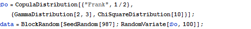 X |
| In[2]:= | 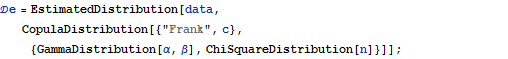 X |
| In[3]:= | 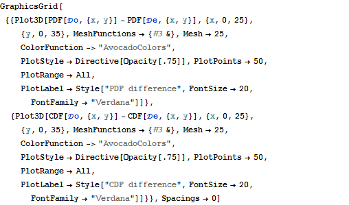 X |
| Out[3]= | 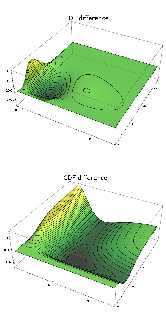 |