핵심 알고리즘

일변량 이산 분포 함수

일변량 이산 분포 함수의 연산 및 시각화를 실행합니다.

In[1]:=

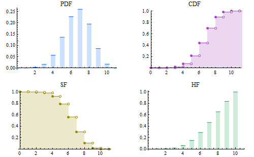
Clear[DistributionPlot];

DistributionPlot[dist_, {xmin_, xmax_}] :=

Block[{k, x, kmin = Floor[xmin], kmax = Ceiling[xmax], pdf, cdf, sf,

hf},

{pdf, cdf, sf, hf} =

{

DiscretePlot[PDF[dist, k], {k, kmin, kmax},

PlotRange -> {{xmin, xmax}, Automatic}, PlotLabel -> "PDF",

PlotStyle -> Hue[.6, 1, 1], Filling -> Axis,

FillingStyle -> Hue[.6, 1, 1], ExtentSize -> 0.5],

DiscretePlot[CDF[dist, k], {k, kmin, kmax}, PlotRange -> {0, 1},

PlotLabel -> "CDF", PlotStyle -> Hue[.8, .7, .8],

Filling -> Axis, FillingStyle -> Hue[.8, .7, .7],

ExtentSize -> Right, ExtentMarkers -> {"Filled", "Empty"}],

DiscretePlot[SurvivalFunction[dist, k], {k, kmin, kmax},

PlotRange -> {0, 1}, PlotLabel -> "SF",

PlotStyle -> Hue[.15, 1, .6], Filling -> Axis,

FillingStyle -> Hue[.15, 1, .6], ExtentSize -> Right,

ExtentMarkers -> {"Filled", "Empty"}],

DiscretePlot[HazardFunction[dist, k], {k, kmin, kmax},

PlotRange -> {{xmin, xmax}, Automatic}, PlotLabel -> "HF",

PlotStyle -> Hue[.4, .7, .6], Filling -> Axis,

FillingStyle -> Hue[.4, 1, .6], ExtentSize -> 0.5]

};

GraphicsGrid[{{pdf, cdf}, {sf, hf}}, ImageSize -> 500]

];

DistributionPlot[BinomialDistribution[10, 2/3], {0, 11}]

Out[1]=