Wolfram
Mathematica
8의 신기능: 웨이블릿 분석
◄
이전
|
다음
►
응용 분야
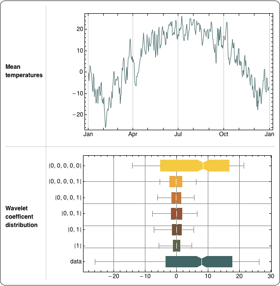
웨이블릿 계수 분포의 시각화
웨이블릿 계수의 범위와 분포를 비교합니다.
In[1]:=
X
data = WeatherData["KMDZ", "MeanTemperature", {{2007, 1, 1}, {2007, 12, 31}, "Day"}];
In[2]:=
X
plot = DateListPlot[data, Joined -> True, ImageSize -> 412, FrameTicksStyle -> Directive[12, FontFamily -> "Helvetica"], PlotStyle -> ColorData["FallColors"][0]];
In[3]:=
X
dwd = StationaryWaveletTransform[data[[All, 2]], HaarWavelet[], 5];
In[4]:=
X
bwc = BoxWhiskerChart[ Join[{data[[All, 2]]}, dwd[Automatic, "Values"]], "Notched", ChartLabels -> Placed[Join[{"data"}, dwd["BasisIndex"]], Axis], BarOrigin -> Left, GridLines -> Automatic, ChartStyle -> "FallColors", ImageSize -> 460, FrameTicksStyle -> Directive[12, FontFamily -> "Helvetica"]];
In[5]:=
X
Framed[Grid[{{Column[{"Mean", "temperatures"}], plot}, {Column[{"Wavelet", "coefficent", "distribution"}], bwc}}, Alignment -> {{Left, Right}, {Center}}, Dividers -> Center, Spacings -> {1, 3}, FrameStyle -> GrayLevel@0.8, BaseStyle -> {FontFamily -> "Helvetica", 12, Bold}], RoundingRadius -> 10, FrameStyle -> GrayLevel@0.2, FrameMargins -> 10]
Out[5]=