imagescale = {Automatic, 500, 128};

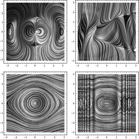
GraphicsGrid[{{LineIntegralConvolutionPlot[{{3*x*y*Cos[Norm[{x, y}]] +

        x*y*Norm[{x, y}]*Sin[Norm[{x, y}]], (2*y^2 - x^2)*

        Cos[Norm[{x, y}]] - x*x*Norm[{x, y}]*Sin[Norm[{x, y}]]}, 

     imagescale}, {x, -Pi, Pi}, {y, -Pi, Pi}, 

    ColorFunction -> GrayLevel, LineIntegralConvolutionScale -> 2, 

    LightingAngle -> Automatic], 

   LineIntegralConvolutionPlot[{{Cos[x^2 + y], 1 + x - y^2}, 

     imagescale}, {x, -3, 3}, {y, -3, 3}, ColorFunction -> GrayLevel, 

    LightingAngle -> 0, 

    LineIntegralConvolutionScale -> 

     3]}, {LineIntegralConvolutionPlot[{{-y, Sin[x]}, 

     imagescale}, {x, -3, 3}, {y, -3, 3}, ColorFunction -> GrayLevel, 

    LightingAngle -> 0, LineIntegralConvolutionScale -> 2], 

   LineIntegralConvolutionPlot[{{-y, Sin[x^3]}, imagescale}, {x, -3, 

     3}, {y, -3, 3}, StreamStyle -> None, ColorFunction -> GrayLevel, 

    LightingAngle -> 0, LineIntegralConvolutionScale -> 2]}}, 

 ImageSize -> Large]