핵심 알고리즘
다변량 비모수 확률과 기대값 추정
이변량 밀도의 PDF는 SmoothKernelDistribution를 이용하여 추정할 수 있으며, 거듭 제곱으로부터 만들어진 데이터와 기대값을 나타낸 것입니다.
| In[1]:= | 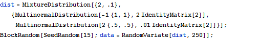 X |
| In[2]:= | X |
| In[3]:= | 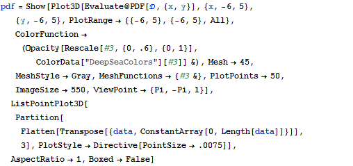 X |
| Out[3]= | 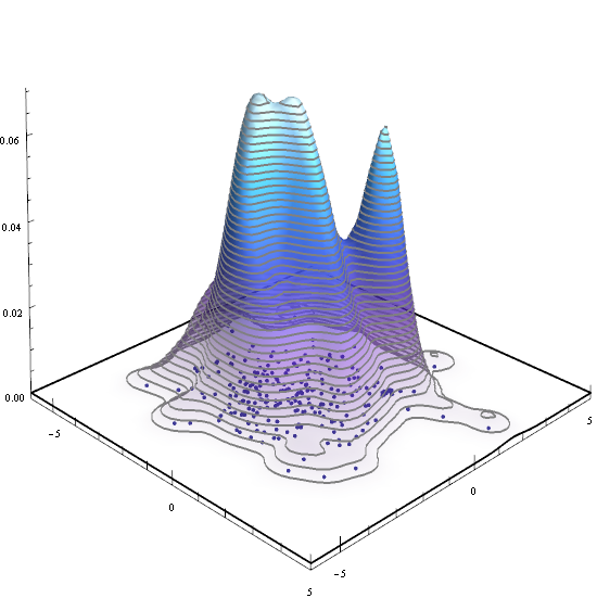 |
| In[4]:= | X |
| In[5]:= | X |
| Out[5]= |
| Wolfram Mathematica 8의 신기능: 비모수 분포, 파생 분포, 포뮬라 분포 | ◄ 이전 | 다음 ► |
| In[1]:= | X |
| In[2]:= | X |
| In[3]:= | X |
| Out[3]= | |
| In[4]:= | X |
| In[5]:= | X |
| Out[5]= |