Examples

Example 1 : Shortest Path

First we define the graph via the nodes and the corresponding costs given in ListOfLinksCosts.

ListOfLinksCosts = {{"a", "b", -1}, {"b", "d", 4}, {"c", "a", 2}, {"c", "b", 3}, {"c", "e", 3}, {"d", "c", 1}, {"d", "e", 2}, {"d", "f", 1}, {"e", "d", -2}, {"e", "f", 0}, {"f", "b", 0}};

The starting node is set to "c" :

We choose the label setting method ("LS"), which is in this case not correct because negative distances occur (e.g., {"a","b",-1}).

{ListOfNodes, ListOfDistanceToStartNode, ListOfPredecessor} = ShortestPathOneToAll[ListOfLinksCosts, StartNode, Method → "LC", PrintOpt → True]; ListOfNodes ListOfDistanceToStartNode ListOfPredecessor

{"a", "b", "c", "d", "e", "f"}

{2, 1, 0, 1, 3, 2}

{"c", "a", "c", "e", "c", "d"}

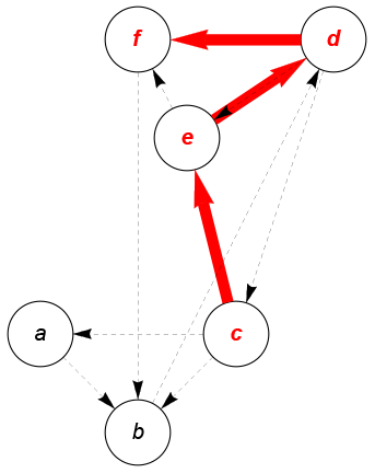
We consider for instance the node "f" as destination, that is, we determine the shortest path from "c" to "f".

TargetNode = "f";

{TotalCosts, ShortestPath} = ConstructShortestPath[ListOfNodes, ListOfDistanceToStartNode, ListOfPredecessor, StartNode, TargetNode]
{2, {"c", "e", "d", "f"}}

The shortest path from "c" to "f" proceeds via e and d, and has length 2.

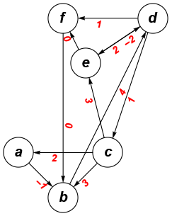
Visualization of the graph may be controlled through the specification of coordinates of the nodes.

Coordinates = {{"a", {0, 0}}, {"b", {3, -3}}, {"c", {6, 0}},{"d", {9, 9}}, {"e", {4.5, 6}}, {"f", {3, 9}}};

The graph has the following representation:

ShowShortestPathInit[ ListOfLinksCosts, Coordinates, PrintWeights → True, PosOfArrowtext → 0.6]

The resulting path (c → f) is visualized as:

ShowShortestPathRes[ ListOfLinksCosts, ShortestPath, Coordinates]

Example 2 : Network Simplex

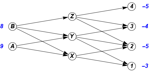
The following small example corresponds to a transport problem with intermediate hubs, that is, nodes that have neither supplies nor demands. In this example, these are the nodes X, Y and Z.

ListOfLinksCapCost = {{A, X, ∞, 1}, {A, Y, ∞, 2}, {B, X, ∞, 3}, {B, Y, ∞, 1}, {B, Z, ∞, 2}, {X, 1, ∞, 5}, {X, 2, 4, 7}, {Y, 1, ∞, 9}, {Y, 2, ∞, 6}, {Y, 3, 3, 7}, {Z, 2, ∞, 8}, {Z, 3, ∞, 10}, {Z, 4, ∞, 4}};

Note the capacity restrictions for some of the connections (X → 2 and Y → 3, resp.).

ListOfSupply = {{A, 9}, {B, 8}, {X, 0}, {Y, 0}, {Z, 0}, {1, -3}, {2, -5}, {3, -4}, {4, -5}};

The graph of the problem is:

ShowNetworkFlowInit[ListOfLinksCapCost, ListOfSupply]

The optimal result is obtained as:

res = NetworkSimplex[ListOfLinksCapCost, ListOfSupply]; TotalCost = res[[1]] Flow = res[[2]]

125

{{A, X, 7}, {A, Y, 2}, {B, Y, 2}, {B, Z, 6}, {X, 1, 3}, {X, 2, 4}, {Y,2, 1}, {Y, 3, 3}, {Z, 3, 1}, {Z, 4, 5}}

And can be visualized also:

ShowNetworkFlowRes[ListOfLinksCapCost, ListOfSupply, res, CircleRadius → 1.5, PosOfArrowtext → 0.5]

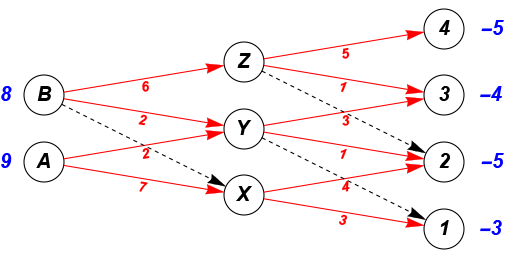
The links that are used for the optimal flow are shown in red, together with the corresponding transport units.