Wolfram Programming Lab is a legacy product.
All the same functionality and features, including access to Programming Lab Explorations, are available with Wolfram|One.
Start programming now. »
All the same functionality and features, including access to Programming Lab Explorations, are available with Wolfram|One.
Start programming now. »
About the Wolfram Language »
Wolfram Programming Lab
Try it now »
(no sign-in required)
(no sign-in required)
Randomness of Pi
Test for randomness in the digits of π.
Run the code to find the numerical value of π to 50 digits. Try getting more than 50 digits—for example, 1,000:
N[Pi, 50]
Get a list of the first 100 digits of π in base 10. Try bases other than 10—for example, 2:
First[RealDigits[Pi, 10, 100]]
Count how often 0 through 9 occur in the first 100 digits. Try more digits than 100:
Counts[First[RealDigits[Pi, 10, 100]]]
Make a bar chart of 0 through 9 frequencies. See if it evens out with more than 100 digits:
BarChart[KeySort[Counts[First[RealDigits[Pi, 10, 100]]]]]
Make a 20×20 array of π digits. Try sizes other than 20—for example, 40:
Grid[With[{n = 20}, Partition[First[RealDigits[Pi, 10, n*n]], n]]]
Visualize the array of digits. Try a larger array than 20×20:
ArrayPlot[
With[{n = 20}, Partition[First[RealDigits[Pi, 10, n*n]], n]]]
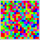
Add color:
ArrayPlot[
With[{n = 20}, Partition[First[RealDigits[Pi, 10, n*n]], n]],
ColorFunction -> Hue]
Make a “π random walk”. Try it for more than 100 digits:
ListLinePlot[Accumulate[First[RealDigits[Pi, 2, 100]] - .5]]
Start programming now (no sign-in required)
Already have a plan? Sign in »