Model Charged Triangular Sheet Field Lines
The Wolfram Language is both a powerful computational language and an efficient language for scientific communication among people. A great example of this is in the entity domain of physical systems. To get a sense of the scope of what is available in "PhysicalSystem", look at a sample of available entities:
Finding a given physical system of interest is simplified by their categorization into entity classes. Currently there are 27 non-disjoint entity classes, of which a sample is shown here.
Rather than containing primarily numerical or textual data, as in, say, the "Country" domain, the physical system domain primarily contains formulas like those one might find in a textbook. To see how these can be used, take the system of interest to be a charged triangular sheet.
A convenient way to see what is available for this entity is by calling "NonMissingProperties".
In general, entities in the "PhysicalSystem" domain are associated with a set of "system variables" that describe the overall physical parameters of the system. For the charged triangular sheet in space, these are the charge,  , of the sheet and the coordinates of its vertices
  for
for  .
.
Any given property may depend on these system variables and possibly on the generalized coordinates of the system. For example, looking to the electric charge density, you have the following.
Note, as is often the case for the formulas returned by "PhysicalSystem", the head of this expression is Inactive[ReplaceRepeated]. This allows for the use of intermediate variables, which can make such expressions smaller and easier to comprehend. For example, in the formula presented earlier,  is the area of the triangle and
  represents the perpendicular distance from the triangle to the measurement point. The DiracDelta and Piecewise pieces represent the fact that the charge density is nonzero only on the (infinitely thin) triangular sheet. Upon activating the replacement, the expression will reduce to one involving only the system variables and generalized coordinates.
A more interesting property to look at might be the electric field of the charged sheet. For simplified visualization, consider sheets in two dimensions (taking  ). The form of the field can be found with the following EntityValue call (the result is suppressed here as is it is somewhat large).
Choosing a triangle of interest, substituting its vertex coordinates into fieldForm and activating yields a straightforward, if complex, closed-form solution for the electric field vector as a function of coordinates in the  -
- plane.
The preceding expression is fairly complicated, so for easier display you can render it in a TraditionalForm Pane.
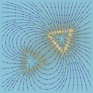
Finally, as a last step, try to visualize the field lines that flow from these formulas. Fortunately, the Wolfram Language has the built-in function StreamDensityPlot for doing just that. You must be a little careful to get rid of the QuantityVariable items in the preceding expression before you can plot it, and the replacements one might use to do this are demonstrated in the following. Additionally, to make a more interesting plot, superimpose two charged triangles and build a Manipulate showing how their fields interact as their relative position, angle and charges are changed. View the code and resulting animation, and enjoy experimenting with simulating physical systems in the Wolfram Language!