Explore a Detailed Model of the Earth's Oceans

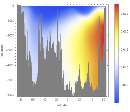
Discover how salinity of seawater deviates at different depths from its standard average value of 35.2 g/kg.

Compute an array of values of salinity anomaly along the 180° E meridian for depths ranging from 0 to 6000 meters, and assuming a constant temperature of 15 °C.

In[1]:=

anomaly = Table[{lat, Quantity[-d, "Meters"], StandardOceanData[<|"Position" -> GeoPosition[{lat, 180}], "Pressure" -> Quantity[d, "Decibars"], "Temperature" -> Quantity[15, "DegreesCelsius"]|>, "AbsoluteSalinityAnomaly"]}, {lat, -85, 65, 5}, {d, 0, 6000, 50}];

The highest deviations are found for larger latitudes.

In[2]:=

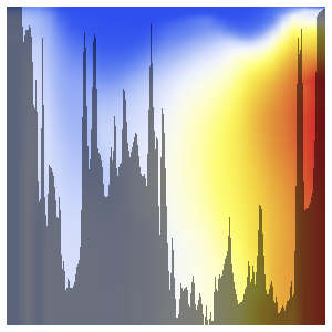
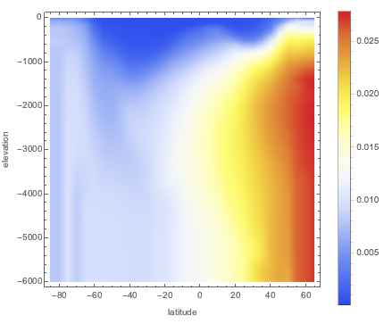
anomalyPlot = ListDensityPlot[Flatten[anomaly, 1], ColorFunction -> "TemperatureMap", FrameLabel -> {"latitude", "elevation"}, PlotLegends -> Automatic, ImageSize -> Medium]

Out[2]=

Superimpose an elevation profile of the sea floor along the same meridian.

In[3]:=

depths = GeoElevationData[ GeoPosition[Table[{lat, 180}, {lat, -85, 65, 1}]], UnitSystem -> "Metric"]; depthsPlot = ListPlot[Transpose[{Range[-85, 65, 1], depths}], Joined -> True, Filling -> Bottom, FillingStyle -> Gray, PlotStyle -> None, Frame -> True, Axes -> False]; Show[anomalyPlot, depthsPlot]

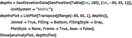
Out[3]=