Wolfram言語™

心臓病データの解析

データ解析は，生のソースから取り出した情報に基づく抽出，表示，モデリングのプロセスである．この例では，Wolfram言語を使ってデータ解析を行うワークフローを示す．ここで使用されるデータ集合は，UCI Machine Learning Repositoryからのもので，1541人の患者の心臓病診断データである．

心臓病診断データをインポートし，各行がそれぞれの患者，各列がさまざまな属性に対応するように，データを構文解析する．

In[1]:=

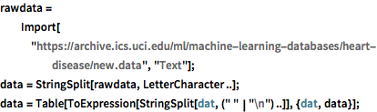
rawdata = Import["https://archive.ics.uci.edu/ml/machine-learning-databases/\ heart-disease/new.data", "Text"]; data = StringSplit[rawdata, LetterCharacter ..]; data = Table[ ToExpression[StringSplit[dat, (" " | "\n") ..]], {dat, data}];

関連のある属性を「labels」と「features」に抽出する．「labels」に入れられた値は0と1であり，それぞれ心臓病の有無に対応する．

In[2]:=

labels = Unitize[data[[All, 58]]]; features = data[[All, {3, 4, 9, 10, 12, 16, 19, 32, 38, 40, 41, 44, 51}]];

In[3]:=

Take[labels, 10]

Out[3]=

それぞれの患者に対して，特徴のベクトルは数値のリストである．しかし，データは完全ではなく，欠測値がとして保存されている．

In[4]:=

features[[-3]]

Out[4]=

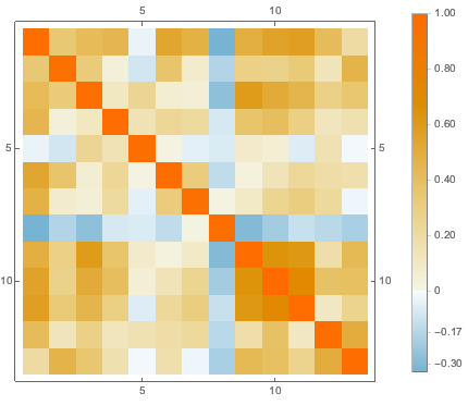
欠測値を，対応する属性内で使用可能なデータの平均で置換してから，さまざまな属性間の相関関係を可視化する．

In[5]:=

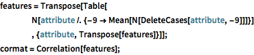
features = Transpose[Table[ N[attribute /. {-9 -> Mean[N[DeleteCases[attribute, -9]]]}] , {attribute, Transpose[features]}]]; cormat = Correlation[features];

In[6]:=

MatrixPlot[cormat, ImageSize -> Medium, PlotTheme -> "Detailed"]

Out[6]=

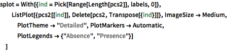
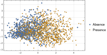
データの分布を可視化するために，PCAを行い，2つの主要なコンポーネントを抽出し，投影されたデータを散布図で表す．

In[7]:=

pcs2 = Take[PrincipalComponents[features, Method -> "Correlation"], All, 2];

In[8]:=

splot = With[{ind = Pick[Range[Length[pcs2]], labels, 0]}, ListPlot[{pcs2[[ind]], Delete[pcs2, Transpose[{ind}]]}, ImageSize -> Medium, PlotTheme -> "Detailed", PlotMarkers -> Automatic, PlotLegends -> {"Absence", "Presence"}] ]

Out[8]=

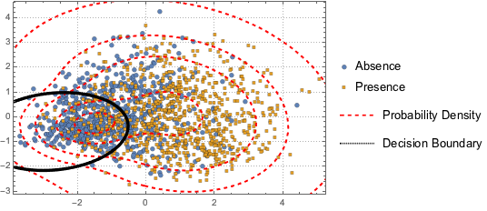
2つのクラスを区別するために，投影されたデータを2つのコンポーネントのガウス混合モデルにフィットする．

In[9]:=

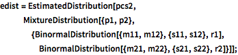
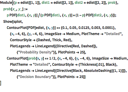
edist = EstimatedDistribution[pcs2, MixtureDistribution[{p1, p2}, {BinormalDistribution[{m11, m12}, {s11, s12}, r1], BinormalDistribution[{m21, m22}, {s21, s22}, r2]}]];

混合モデルに基づき，混合モデルの決定境界（黒の曲線）と確率密度等高線（赤の曲線）をプロットし，散布図に重ね合せて表示する．ガウス混合モデルの1つ目のコンポーネントの方が決定境界内で高い確率を持つ．

In[10]:=

Module[{p = edist[[1, 1]], dist1 = edist[[2, 1]], dist2 = edist[[2, 2]], prob}, prob[x_, y_] := p PDF[dist1, {x, y}]/(p PDF[dist1, {x, y}] + (1 - p) PDF[dist2, {x, y}]); Show[splot, ContourPlot[ PDF[edist, {x, y}] == {0.1, 0.05, 0.0125, 0.003, 0.0001}, {x, -4, 6}, {y, -4, 6}, ImageSize -> Medium, PlotTheme -> "Detailed", ContourStyle -> {Dashed, Thick, Red}, PlotLegends -> LineLegend[{Directive[Red, Dashed]}, {"Probability Density"}], PlotPoints -> 25], ContourPlot[prob[x, y] == 1/2, {x, -4, 6}, {y, -4, 6}, ImageSize -> Medium, PlotTheme -> "Detailed", ContourStyle -> {Thickness[.01], Black}, PlotLegends -> LineLegend[{Directive[Black, AbsoluteDashing[{1, 1}]]}, {"Decision Boundary"}], PlotPoints -> 25]] ]

Out[10]=