利用 DTW 比较股票价格: Wolfram语言 11 的新功能

利用 DTW 比较股票价格

利用 WarpingCorrespondence 对 HPQ 股票 2016 年第一季度的数据和 2010 到 2015 年的历史数据进行比较.

In[1]:=

recent = FinancialData["HPQ", {{2016, 1, 1}, {2016, 3, 31}}, 
   "Value"];
{histDates, hist} = 
  Transpose[
   FinancialData["HPQ", {{2010, 1, 1}, {2015, 1, 31}}, "DateValue"]];

求与之最相似的历史数据.

In[2]:=

{corrHist, corrRecent} = 
  WarpingCorrespondence[hist, recent, 
   Method -> {"MatchingInterval" -> "Flexible"}];

查找与 2016 年第一季度最相似的历史时段.

In[3]:=

{m, n} = corrHist[[{1, -1}]];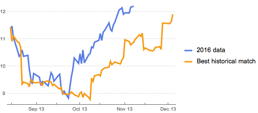
histDates[[{m, n}]]

Out[3]=

可视化最近的数据与最相似的历史数据.

显示完整的 Wolfram 语言输入

In[4]:=

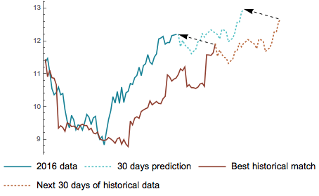
DateListPlot[{AssociationThread[
   Take[histDates[[m ;; n]], Length[recent]], recent], 
  AssociationThread[histDates[[m ;; n]], hist[[m ;; n]]]}, 
 PlotTheme -> "Business", 
 PlotLegends -> {"2016 data", "Best historical match"}, 
 DateTicksFormat -> {"MonthNameShort", " ", "YearShort"},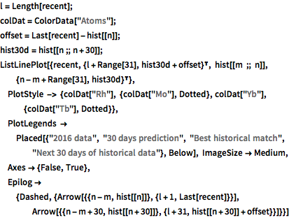 
 ImageSize -> Medium]

Out[4]=

根据历史数据预测接下来 30 天的股票价格.

显示完整的 Wolfram 语言输入

In[5]:=

l = Length[recent];
colDat = ColorData["Atoms"];
offset = Last[recent] - hist[[n]];
hist30d = hist[[n ;; n + 30]];
ListLinePlot[{recent, {l + Range[31], hist30d + offset}\[Transpose], 
  hist[[m ;; n]], {n - m + Range[31], hist30d}\[Transpose]}, 
 PlotStyle -> {colDat["Rh"], {colDat["Mo"], Dotted}, 
   colDat["Yb"], {colDat["Tb"], Dotted}}, 
 PlotLegends -> 
  Placed[{"2016 data", "30 days prediction", "Best historical match", 
    "Next 30 days of historical data"}, Below], ImageSize -> Medium, 
 Axes -> {False, True}, 
 Epilog -> {Dashed, {Arrow[{{n - m, hist[[n]]}, {l + 1, 
       Last[recent]}}], 
    Arrow[{{n - m + 30, hist[[n + 30]]}, {l + 31, 
       hist[[n + 30]] + offset}}]}}]

Out[5]=

Wolfram 语言™

利用 DTW 比较股票价格

相关范例