Wolfram Language™

Trends and Seasonalities

The number of airline passengers in years 1949 to 1960 was increasing but also varied seasonally. Apply MovingMap with Total over non-overlapping yearly windows to visualize annual growth. Use DateHistogram for monthly data with yearly date reduction to study seasonal dependencies.

The number of international airline passengers per month in years 1949 to 1960 is available via ExampleData.

In[1]:=

data = ExampleData[{"Statistics", "InternationalAirlinePassengers"}, "TimeSeries"]

Out[1]=

The data exhibits both a long-term increasing trend and seasonal oscillations.

In[2]:=

DateListPlot[data, PlotTheme -> "Detailed"]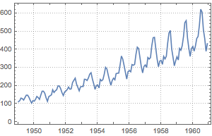

Out[2]=

Aggregate yearly to see the global trend. Place the aggregated results at the last day of each year to make the 1-year moving windows non-overlapping.

In[3]:=

positionspec = {{1949, 12, 31}, {1960, 12, 31}, Quantity[1, "Year"]};

In[4]:=

mm = MovingMap[Total, data, {Quantity[1, "Years"], Right, positionspec}];

In[5]:=

DateListPlot[mm, PlotMarkers -> Automatic, GridLines -> {mm["Dates"], None}]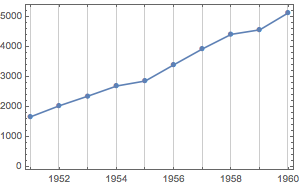

Out[5]=

Analyze seasonal dependence. Create WeightedData with number of passengers as weights for the dates.

In[6]:=

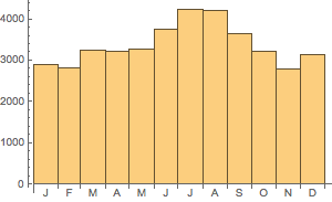
wd = WeightedData[data["Dates"], data["Values"]];

DateHistogram aggregates the weights for each month over the years as specified by DateReduction.

In[7]:=

DateHistogram[wd, "Month", DateReduction -> "Year"]

Out[7]=