Approximate Signal Derivative

Use MovingMap to approximate the derivative of a signal coming from irregularly sampled continuous time series.

In[1]:=

ts = TimeSeries[ Table[{t, EllipticTheta[1, t, 0.3]}, {t, Join[{0.}, RandomReal[{0, 2 Pi}, 254], {2. Pi}]}]]

Out[1]=

In[2]:=

RegularlySampledQ[ts]

Out[2]=

In[3]:=

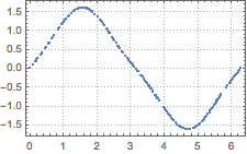
ListPlot[ts, PlotTheme -> "Detailed"]

Out[3]=

Use the values and the times at the boundaries of each sliding window to compute the difference quotients.

In[4]:=

quotient[values_, times_] := First[Differences[values]/Differences[times]]

In[5]:=

mm = MovingMap[quotient[#BoundaryValues, #BoundaryTimes] &, ts, {.01, Right}]

Out[5]=

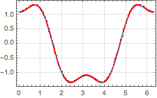
Compare to the theoretical derivative.

In[6]:=

prime = D[EllipticTheta[1, t, 0.3], t]

Out[6]=

In[7]:=

Show[Plot[prime, {t, 0, 2 \[Pi]}, PlotStyle -> Thick, PlotTheme -> "Detailed", PlotLegends -> None], ListPlot[mm, PlotStyle -> Red]]

Out[7]=

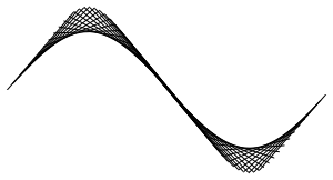
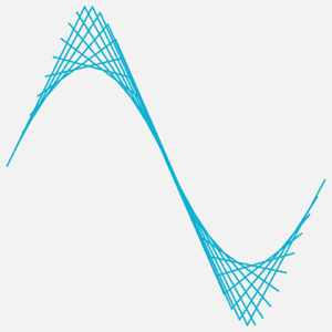
Use MovingMap with Line in place of the quotient function to create a plot of secant lines that approximate the original time series.

In[8]:=

line[yvals_, xvals_] := Line[Transpose[{xvals, yvals}]];

In[9]:=

lines = MovingMap[ line[#BoundaryValues, #BoundaryTimes] &, ts, {1.3, Right, {0, 2. \[Pi], .1}}];

In[10]:=

Graphics[{Black, lines["Values"]}]

Out[10]=