Wolfram言語™

数量配列

QuantityArrayは，Quantityオブジェクトの配列の効率的な保存と操作を可能にし，物理単位を持つデータの解析に理想的である．系を通しての積分を続けることで，いくつかの関数がQuantityArrayオブジェクトを理解し，返すようになった．

QuantityDistributionオブジェクトからサンプルを取る．

In[1]:=

RandomVariate[ParetoDistribution[Quantity[500., "USDollars"], 4], 300]

Out[1]=

QuantityArrayオブジェクトはQuantity要素の正規配列と同じである．

In[2]:=

RandomVariate[ParetoDistribution[Quantity[500., "USDollars"], 4], 300]; Normal[Take[%, 10]]

Out[2]=

高度データや磁場データのような地理データを計算あるいはダウンロードする．

In[3]:=

GeoElevationData[Entity["Country", "UnitedStates"]]

Out[3]=

In[4]:=

GeomagneticModelData[ Entity["GeographicRegion", "Antarctica"], "Magnitude"]

Out[4]=

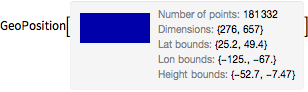
経緯度角の配列を操作する．

In[5]:=

GeoElevationData[ Entity["Country", "UnitedStates"], "Undulation", GeoPosition]

Out[5]=

In[6]:=

GeoElevationData[ Entity["Country", "UnitedStates"], "Undulation", GeoPosition]; LatitudeLongitude[%]

Out[6]=

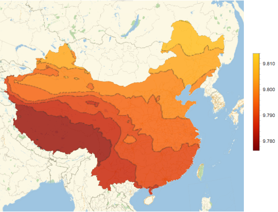
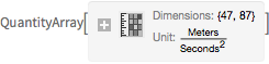
中国の重力場についての垂直成分のデータ配列を取得する．

In[7]:=

data = GeogravityModelData[Entity["Country", "China"], "DownComponent"]

Out[7]=

この地域の地球の重力場が標準の9.81とどのように異なるかを調べる．

In[8]:=

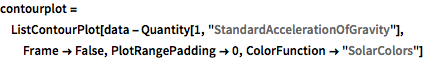
contourplot = ListContourPlot[data - Quantity[1, "StandardAccelerationOfGravity"], Frame -> False, PlotRangePadding -> 0, ColorFunction -> "SolarColors"]

Out[8]=

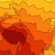
中国の地図に等高線プロットを重ねる．

In[9]:=

Legended[GeoGraphics[{GeoStyling[{"GeoImage", contourplot}, Opacity[0.8]], Polygon[Entity["Country", "China"]]}, ImageSize -> 500, GeoRange -> Quantity[2200, "Kilometers"], GeoZoomLevel -> 5], BarLegend[{"SolarColors", MinMax@Flatten[QuantityMagnitude@data]}]]

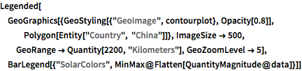
Out[9]=