可视化飓风数据: Wolfram语言 11 的新功能

‹›

可视化飓风数据

一个涡旋的简单模型由一个核心内的旋转体加上逐渐减小的外层角速度组合而成.

显示完整的 Wolfram 语言输入

In[1]:=

w = 6; rcore = 3; a = 1; g = 9.82; rho = 1; Subscript[rho, 0] = 1;

In[2]:=

wind[r_, z_] := If[r <= rcore, w r, (w a^2)/r];

由计算压强的公式给出下面用半径和海拔表示的公式.

In[3]:=

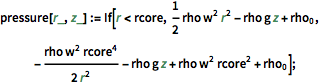
pressure[r_, z_] := 
  If[r < rcore, 
   1/2 rho w^2 r^2 - rho g z + Subscript[rho, 
    0], -((rho w^2 rcore^4)/(2 r^2)) - rho g z + rho w^2 rcore^2 + 
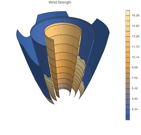
    Subscript[rho, 0]];

绘制风速图形，风速在系统的中心外侧最快.

In[4]:=

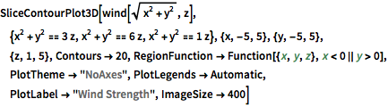
SliceContourPlot3D[
 wind[Sqrt[x^2 + y^2], z], {x^2 + y^2 == 3 z, x^2 + y^2 == 6 z, 
  x^2 + y^2 == 1 z}, {x, -5, 5}, {y, -5, 5}, {z, 1, 5}, 
 Contours -> 20, 
 RegionFunction -> Function[{x, y, z}, x < 0 || y > 0], 
 PlotTheme -> "NoAxes", PlotLegends -> Automatic, 
 PlotLabel -> "Wind Strength", ImageSize -> 400]

Out[4]=

以矢量场的形式画出风向.

In[5]:=

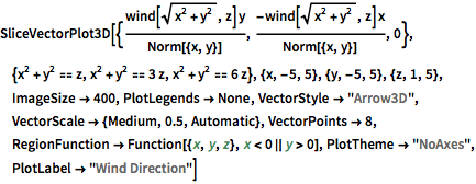
SliceVectorPlot3D[{(wind[Sqrt[x^2 + y^2], z] y)/
  Norm[{x, y}], (-wind[Sqrt[x^2 + y^2], z] x)/Norm[{x, y}], 
  0}, {x^2 + y^2 == z, x^2 + y^2 == 3 z, x^2 + y^2 == 6 z}, {x, -5, 
  5}, {y, -5, 5}, {z, 1, 5}, ImageSize -> 400, PlotLegends -> None, 
 VectorStyle -> "Arrow3D", VectorScale -> {Medium, 0.5, Automatic}, 
 VectorPoints -> 8, 
 RegionFunction -> Function[{x, y, z}, x < 0 || y > 0], 
 PlotTheme -> "NoAxes", PlotLabel -> "Wind Direction"]

Out[5]=

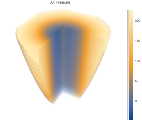
画出压强的三维密度图. 注意在系统中心相对较低的压强.

In[6]:=

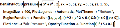
DensityPlot3D[
 pressure[Sqrt[x^2 + y^2], z], {x, -5, 5}, {y, -5, 5}, {z, 1, 5}, 
 ImageSize -> 400, PlotLegends -> Automatic, PlotTheme -> "NoAxes", 
 RegionFunction -> 
  Function[{x, y, z}, (x^2 + y^2 <= 6 z) && (x < 0 || y > 0)], 
 PlotLabel -> "Air Pressure", 
 OpacityFunction -> Function[f, f/5 + 0.1]]

Out[6]=

Wolfram 语言™

可视化飓风数据

相关范例