Observe a Quantum Particle in a Box
A quantum particle free to move within a two-dimensional rectangle with sides  and
and  is described by the two-dimensional time-dependent Schrödinger equation, together with boundary conditions that force the wavefunction to zero at the boundary.
eqn = I D[\[Psi][x, y, t], t] == -\[HBar]^2/(2 m)
Laplacian[\[Psi][x, y, t], {x, y}];bcs = {\[Psi][0, y, t] == 0, \[Psi][xMax, y, t] ==
0, \[Psi][x, yMax, t] == 0, \[Psi][x, 0, t] == 0};This equation has a general solution that is a formal infinite sum of so-called eigenstates.
DSolveValue[{eqn, bcs}, \[Psi][x, y, t], {x, y, t}]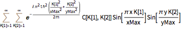
Define an initial condition equal to a unitized eigenstate.
initEigen = \[Psi][x, y, 0] ==
   2 /Sqrt[xMax yMax] Sin[(\[Pi] x)/xMax] Sin[(\[Pi] y)/yMax];
In this case, the solution is simply a time-dependent multiple (of unit modulus) of the initial condition.
DSolveValue[{eqn, bcs, initEigen}, \[Psi][x, y, t], {x, y, t}]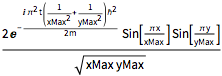
Define an initial condition that is a sum of eigenstates. Because the initial conditions are not an eigenstate, the probability density for the location of the particle will be time dependent.
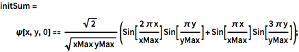
initSum = \[Psi][x, y, 0] ==
   Sqrt[2]/Sqrt[
    xMax yMax] (Sin[(2 \[Pi] x)/xMax] Sin[(\[Pi] y)/yMax] +
      Sin[(\[Pi] x)/xMax] Sin[(3 \[Pi] y)/yMax]);
Solve with the new initial condition.
sol = DSolveValue[{eqn, bcs, initSum}, \[Psi][x, y, t], {x, y, t}]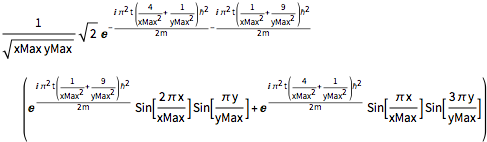
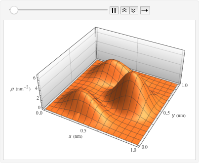
Compute the probability density, inserting values of the reduced Planck's constant, electron mass, and a box of atomic size, using units of the electron mass, nanometers, and femtoseconds.
\[HBar] =
 QuantityMagnitude[Quantity[1., "ReducedPlanckConstant"],
"ElectronMass" * ("Nanometers")^2/"Femtoseconds"]\[Rho][x_, y_, t_] =
FullSimplify[ComplexExpand[Conjugate[sol] sol]] /. {m -> 1,
xMax -> 1, yMax -> 1}Visualize the probability density inside the box over time.
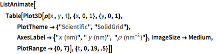
ListAnimate[
 Table[Plot3D[\[Rho][x , y , t], {x, 0, 1}, {y, 0, 1},
   PlotTheme -> {"Scientific", "SolidGrid"}, AxesLabel -> {"\!\(\*
StyleBox[\"x\", \"SO\"]\) (nm)", " \!\(\*
StyleBox[\"y\", \"SO\"]\) (nm)", "\!\(\*
StyleBox[\"\[Rho]\", \"SO\"]\) (\!\(\*SuperscriptBox[\(nm\), \
\(-2\)]\))"}, ImageSize -> Medium, PlotRange -> {0, 7}], {t, 0,
   19, .5}]]