Compute Sensitivities of PDEs over Regions
Compute the parametric dependence of the wave equation  ,
,  .
.
Specify the wave equation 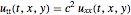 .
.
In[1]:=
eqn = D[u[t, x, y], t, t] == c^2 Laplacian[u[t, x, y], {x, y}];Specify initial conditions  .
.
In[2]:=
ics = {u[0, x, y] == Exp[-((a x)^2 + (b x)^2)],
   Derivative[1, 0, 0][u][0, x, y] == 0};
Specify a fixed Dirichlet boundary condition.
In[3]:=
bcs = DirichletCondition[u[t, x, y] == 0, True];Set up the parametric function.
In[4]:=
pfun = ParametricNDSolveValue[{eqn, ics, bcs},
   u, {t, 0, 5}, {x, y} \[Element] Disk[], {a, b, c}];
Find the sensitivities  ,
,  , and
, and  for parameters
  ,
,  , and
, and  .
.
In[5]:=
ifda = D[pfun[a, 1, 1], a] /. {a -> 1};
ifda = D[pfun[1, b, 1], b] /. {b -> 1};
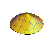
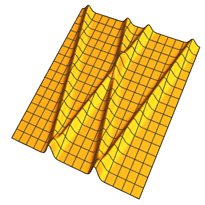
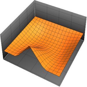
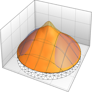
ifdc = D[pfun[1, 1, c], c] /. {c -> 1};Visualize the corresponding sensitivity bands by plotting the parametric function for  ,
,  , and
, and  at
at  and overlaying the solution with
  of the sensitivity.
In[6]:=
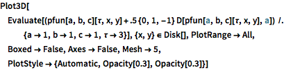
Plot3D[Evaluate[(pfun[a, b, c][\[Tau], x,
      y] + .5 {0, 1, -1} D[pfun[a, b, c][\[Tau], x, y], a]) /. {a ->
     1, b -> 1, c -> 1, \[Tau] -> 3}], {x, y} \[Element] Disk[],
 PlotRange -> All, Boxed -> False, Axes -> False, Mesh -> 5,
 PlotStyle -> {Automatic, Opacity[0.3], Opacity[0.3]}]
Out[6]=