数量数据的非参数化分布
利用 WeatherData 获取芝加哥市从 2014 年初到 2015 年末的风速测量的时间序列.
In[1]:=
wsts = WeatherData["Chicago",
  "WindSpeed", {DateObject[{2014, 1, 1}], DateObject[{2015, 12, 31}]}]
Out[1]=
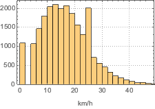
用 Histogram 来可视化风速的分布.
In[2]:=
Histogram[wsts, PlotTheme -> "Detailed", FrameLabel -> Automatic]Out[2]=
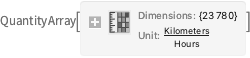
提取风速值,用插值法补齐缺失数据.
In[3]:=
winds = Values[TimeSeries[wsts, MissingDataMethod -> "Interpolation"]]Out[3]=
用 SmoothKernelDistribution 构建芝加哥市风速的非参数化模型,要确保风速不能是负值.
In[4]:=
ws\[ScriptCapitalD] =
 SmoothKernelDistribution[winds,
  Automatic, {"Bounded", Quantity[0, ("Kilometers")/("Hours")],
   "Gaussian"}]
Out[4]=
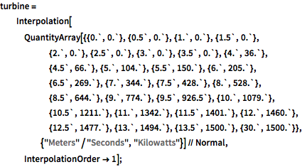
用作为风速的函数的风力发电机功率输出的非参数化模型,来估计安装在当地的 GE 1.5 兆瓦风力发电机的平均输出功率.
In[5]:=
turbine =
  Interpolation[
   QuantityArray[{{0.`, 0.`}, {0.5`, 0.`}, {1.`, 0.`}, {1.5`,
       0.`}, {2.`, 0.`}, {2.5`, 0.`}, {3.`, 0.`}, {3.5`, 0.`}, {4.`,
       36.`}, {4.5`, 66.`}, {5.`, 104.`}, {5.5`, 150.`}, {6.`,
       205.`}, {6.5`, 269.`}, {7.`, 344.`}, {7.5`, 428.`}, {8.`,
       528.`}, {8.5`, 644.`}, {9.`, 774.`}, {9.5`, 926.5`}, {10.`,
       1079.`}, {10.5`, 1211.`}, {11.`, 1342.`}, {11.5`,
       1401.`}, {12.`, 1460.`}, {12.5`, 1477.`}, {13.`,
       1494.`}, {13.5`, 1500.`}, {30.`, 1500.`}}, {"Meters"/"Seconds",
       "Kilowatts"}] // Normal, InterpolationOrder -> 1];
In[6]:=
NExpectation[turbine[v], v \[Distributed] ws\[ScriptCapitalD]]Out[6]=