수량 데이터의 비모수 분포
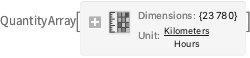
WeatherData를 사용하여 2014년 초부터 2015년 말까지 시카고에서 측정 된 풍속의 시계열을 얻습니다.
In[1]:=
wsts = WeatherData["Chicago",
  "WindSpeed", {DateObject[{2014, 1, 1}], DateObject[{2015, 12, 31}]}]
Out[1]=
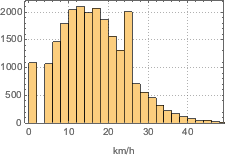
Histogram을 사용하여 풍속의 분포를 시각화합니다.
In[2]:=
Histogram[wsts, PlotTheme -> "Detailed", FrameLabel -> Automatic]Out[2]=
결측치를 보간하여 풍속 값을 추출합니다.
In[3]:=
winds = Values[TimeSeries[wsts, MissingDataMethod -> "Interpolation"]]Out[3]=
SmoothKernelDistribution을 사용하여 반드시 풍속을 비음으로하여 시카고의 풍속 비모수 모델을 구축합니다.
In[4]:=
ws\[ScriptCapitalD] =
 SmoothKernelDistribution[winds,
  Automatic, {"Bounded", Quantity[0, ("Kilometers")/("Hours")],
   "Gaussian"}]
Out[4]=
터빈의 전력 출력의 비모수 모델을 풍속 함수로 사용하여 그 장소에 설치된 GE 1.5 MW 바람 터빈의 평균 전력 출력을 추정합니다.
In[5]:=
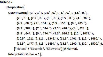
turbine =
  Interpolation[
   QuantityArray[{{0.`, 0.`}, {0.5`, 0.`}, {1.`, 0.`}, {1.5`,
       0.`}, {2.`, 0.`}, {2.5`, 0.`}, {3.`, 0.`}, {3.5`, 0.`}, {4.`,
       36.`}, {4.5`, 66.`}, {5.`, 104.`}, {5.5`, 150.`}, {6.`,
       205.`}, {6.5`, 269.`}, {7.`, 344.`}, {7.5`, 428.`}, {8.`,
       528.`}, {8.5`, 644.`}, {9.`, 774.`}, {9.5`, 926.5`}, {10.`,
       1079.`}, {10.5`, 1211.`}, {11.`, 1342.`}, {11.5`,
       1401.`}, {12.`, 1460.`}, {12.5`, 1477.`}, {13.`,
       1494.`}, {13.5`, 1500.`}, {30.`, 1500.`}}, {"Meters"/"Seconds",
       "Kilowatts"}] // Normal, InterpolationOrder -> 1];
In[6]:=
NExpectation[turbine[v], v \[Distributed] ws\[ScriptCapitalD]]Out[6]=