用地磁场建模绘制西北航道图: Wolfram 语言 11 的新功能

用地磁场建模绘制西北航道图

西北航道是沿北美海岸的海上航道，其连通了北大西洋和太平洋. 该航道在1850 年发现并由探险家罗尔德·阿蒙森在1903年–1906年进行了首次航行. 由于在高纬度磁北和真北相差很大，使用传统磁罗盘在西北航道上航行非常具有挑战性. 该范例通过用 GeomagneticModelData 给出地球当前的磁场数据描绘出西北航道航线.

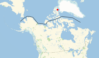
首先使用描述西北航道经纬度组的列表，并获取磁北的位置.

In[1]:=

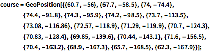
course = GeoPosition[{{60.7, -56}, {67.7, -58.5}, {74, -74.4}, {74.4, \
-91.8}, {74.3, -95.9}, {74.2, -98.5}, {73.7, -113.5}, {73.08, \
-116.86}, {72.57, -118.9}, {71.29, -119.9}, {70.7, -124.3}, {70.83, \
-128.4}, {69.85, -139.6}, {70.44, -143.1}, {71.6, -156.5}, {70.4, \
-163.2}, {68.9, -167.3}, {65.7, -168.5}, {62.3, -167.9}}];

In[2]:=

geomagneticNorthLocation = 
 GeomagneticModelData["NorthGeomagneticPole"]

Out[2]=

In[3]:=

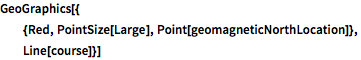
GeoGraphics[{
  {Red, PointSize[Large], Point[geomagneticNorthLocation]},
  Line[course]}]

Out[3]=

定义函数来绘制磁北极（红色）方向和本地罗盘测量值（蓝色）.

In[4]:=

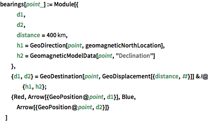
bearings[point_] := Module[{
   d1,
   d2,
   distance = Quantity[400, "Kilometers"],
   h1 = GeoDirection[point, geomagneticNorthLocation],
   h2 = GeomagneticModelData[point, "Declination"]
   },
  {d1, d2} = 
   GeoDestination[point, GeoDisplacement[{distance, #}]] & /@ {h1, h2};
  {Red, Arrow[{GeoPosition@point, d1}], Blue, 
   Arrow[{GeoPosition@point, d2}]}
  ]

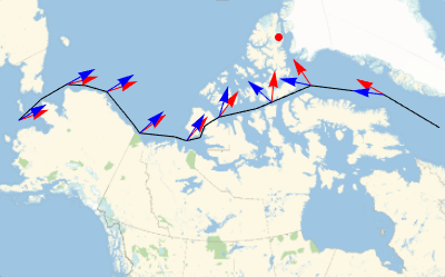
选取间隔合适的样本点集合，通过视觉观察沿航道的真北（红色）和磁北（蓝色）的差别.

In[5]:=

samplepoints = course[[All, {2, 3, 4, 7, 11, 13, 15, 17, 19}]];

In[6]:=

GeomagneticModelData[#, "Declination"] & /@ Thread[samplepoints]

Out[6]=

In[7]:=

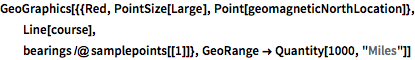
GeoGraphics[{{Red, PointSize[Large], Point[geomagneticNorthLocation]},
   Line[course],
  bearings /@ samplepoints[[1]]}, GeoRange -> Quantity[1000, "Miles"]]

Out[7]=

Wolfram 语言™

用地磁场建模绘制西北航道图

相关范例