Wolfram Language

Richer Knowledgebase Access

Explore Movieology

Use the Wolfram Knowledgebase to study the per minute cost and box office receipts for films released since the year 2000. Additionally, explore the average runtime of these films, which, unusually among humanmade objects, appears to follow a so-called stable distribution law.

Use an implicitly defined entity class to select movies released since the turn of the millennium.
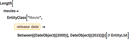
In[1]:=
Click for copyable input
Length[movies = EntityClass["Movie", EntityProperty["Movie", "ReleaseDate"] -> Between[{DateObject[{2000}], DateObject[{2015}]}]] // EntityList]
Out[1]=

Retrieve the movie titles, genres, runtimes, production budgets, and box office totals.
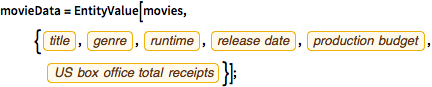
In[2]:=
Click for copyable input
movieData = EntityValue[ movies, {EntityProperty["Movie", "Name"], EntityProperty["Movie", "Genres"], EntityProperty["Movie", "Runtime"], EntityProperty["Movie", "ReleaseDate"], EntityProperty["Movie", "ProductionBudget"], 
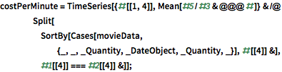
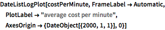
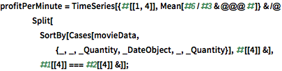
EntityProperty["Movie", "DomesticBoxOfficeGross"]}];

The cost per minute of a released movie is a highly fluctuating function over time.

show complete Wolfram Language input
In[3]:=
Click for copyable input
costPerMinute = TimeSeries[{#[[1, 4]], Mean[#5/#3 & @@@ #]} & /@ Split[SortBy[ Cases[movieData, {_, _, _Quantity, _DateObject, _Quantity, _}], \ #[[4]] &], #1[[4]] === #2[[4]] &]];
In[4]:=
Click for copyable input
DateListLogPlot[costPerMinute, FrameLabel -> Automatic, PlotLabel -> "average cost per minute", AxesOrigin -> {DateObject[{2000, 1, 1}], 0}]
Out[4]=

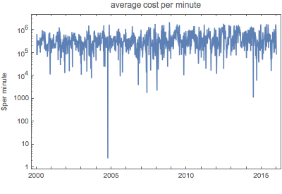
However, averaged over a month, some cost per minute periodicities become visible. In particular, the green grid lines denote the Fourth of July and the purple lines Thanksgiving in the following plot.

show complete Wolfram Language input
In[5]:=
Click for copyable input
DateListPlot[MovingAverage[costPerMinute, Quantity[1, "Months"]], FrameLabel -> Automatic, PlotLabel -> "average cost per minute", AxesOrigin -> {DateObject[{2000, 1, 1}], 0}, GridLines -> {Join[{#, Darker[Green]} & /@ Table[DateObject[{y, 7, 4}], {y, 2000, 2015}], {#, Darker[Purple]} & /@ Table[DateObject@ WolframAlpha[ "Thanksgiving " <> IntegerString[y], {{"Result", 1}, "ComputableData"}], {y, 2000, 2015}]], None}]
Out[5]=

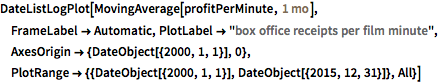
As shown in the following logarithmic plot, box office receipts per minute are an even more wildly fluctuating function.

show complete Wolfram Language input
In[6]:=
Click for copyable input
profitPerMinute = TimeSeries[{#[[1, 4]], Mean[#6/#3 & @@@ #]} & /@ Split[SortBy[ Cases[movieData, {_, _, _Quantity, _DateObject, _, _Quantity}], \ #[[4]] &], #1[[4]] === #2[[4]] &]];
In[7]:=
Click for copyable input
DateListLogPlot[MovingAverage[profitPerMinute, Quantity[1, "Months"]], FrameLabel -> Automatic, PlotLabel -> "box office receipts per film minute", AxesOrigin -> {DateObject[{2000, 1, 1}], 0}, PlotRange -> {{DateObject[{2000, 1, 1}], DateObject[{2015, 12, 31}]}, All}]
Out[7]=

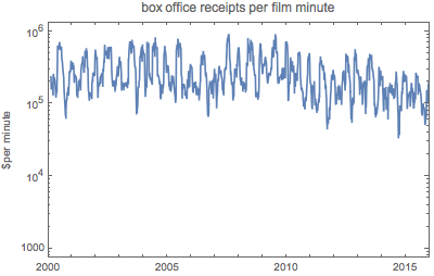
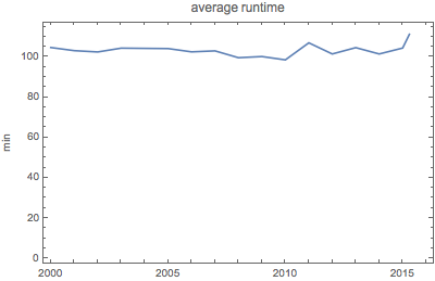
The average runtime of the movies has been fairly consistent over the last 15 years.

show complete Wolfram Language input
In[8]:=
Click for copyable input
averageRuntimes = {#[[1, 1]], Mean[#[[All, -1]]]} & /@ Split[Sort[{DateObject[{#4["Year"]}], UnitConvert[#3, "Minutes"]} & @@@ Cases[movieData, {_, _, _Quantity, _DateObject, _, _}]], #1[[ 1]] === #2[[1]] &];
In[9]:=
Click for copyable input
DateListPlot[averageRuntimes, FrameLabel -> Automatic, PlotLabel -> "average runtime", AxesOrigin -> {DateObject[{2000, 1, 1}], 0}]
Out[9]=

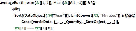
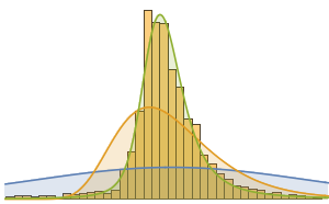
Looking in more detail, the distribution of the movie runtimes appears relatively smooth.

In[10]:=
Click for copyable input
movieRuntimes = DeleteMissing[movieData[[All, 3]]];
In[11]:=
Click for copyable input
hg = Histogram[movieRuntimes, {1, 200, 5}, "PDF", AxesLabel -> Automatic]
Out[11]=

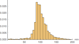
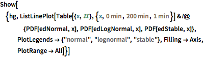
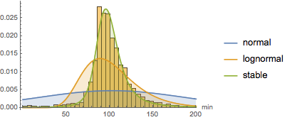
Modeling using a large number of built-in distributions indicates that the closest fit is provided by a Lévy stable distribution. Here, fits using a normal (distribution of the averages of random variables independently drawn from independent distributions), lognormal (the distribution of the multiplicative product of many independent positive random variables), and a stable distribution are computed.

In[12]:=
Click for copyable input
edNormal = EstimatedDistribution[movieRuntimes, NormalDistribution[\[Mu], \[Sigma]]]
Out[12]=
In[13]:=
Click for copyable input
edLogNormal = EstimatedDistribution[movieRuntimes, LogNormalDistribution[\[Mu], \[Sigma]]]
Out[13]=
In[14]:=
Click for copyable input
edStable = EstimatedDistribution[movieRuntimes, StableDistribution[1, \[Alpha], \[Beta], \[Mu], \[Sigma]]]
Out[14]=

Interestingly, the stable distribution is visually the best fit.
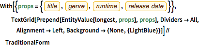
show complete Wolfram Language input
In[15]:=
Click for copyable input
Show[{hg, ListLinePlot[ Table[{x, #}, {x, Quantity[0, "Minutes"], Quantity[200, "Minutes"], Quantity[1, "Minutes"]}] & /@ {PDF[edNormal, x], PDF[edLogNormal, x], PDF[edStable, x]}, PlotLegends -> {"normal", "lognormal", "stable"}, Filling -> Axis, PlotRange -> All]}]
Out[15]=

Only a few humanmade objects obey a stable distribution. One characteristic feature of a stable distribution is the occurrence of relatively large outliers, often a few times larger than the mean. This characteristic is fulfilled by movies. Here, an implicitly defined entity class is used to select the 10 longest (by running time) movies released after January 1, 2000.
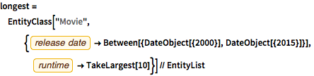
In[16]:=
Click for copyable input
longest = EntityClass[ "Movie", {EntityProperty["Movie", "ReleaseDate"] -> Between[{DateObject[{2000}], DateObject[{2015}]}], EntityProperty["Movie", "Runtime"] -> TakeLargest[10]}] // EntityList
Out[16]=

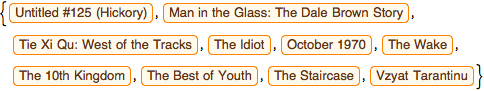
Summarize in a grid.

show complete Wolfram Language input
In[17]:=
Click for copyable input
With[{props = {EntityProperty["Movie", "Name"], EntityProperty["Movie", "Genres"], EntityProperty["Movie", "Runtime"], EntityProperty["Movie", "ReleaseDate"]}}, TextGrid[Prepend[EntityValue[longest, props], props], Dividers -> All, Alignment -> Left, Background -> {None, {LightBlue}}]] // TraditionalForm
Out[17]//TraditionalForm=

Related Examples

de es fr ja ko pt-br ru zh