Solve a Wave Equation with Periodic Boundary Conditions
Solve a 1D wave equation with periodic boundary conditions.
Specify a wave equation with absorbing boundary conditions. Note that the Neumann value is for the first time derivative of  .
.
In[1]:=
eqn = D[u[t, x], {t, 2}] ==
   D[u[t, x], {x, 2}] +
    NeumannValue[-Derivative[1, 0][u][t, x], x == 0 || x == 1];
Specify initial conditions for the wave equation.
In[2]:=
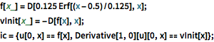
f[x_] = D[0.125 Erf[(x - 0.5)/0.125], x];
vInit[x_] = -D[f[x], x];
ic = {u[0, x] == f[x], Derivative[1, 0][u][0, x] == vInit[x]};
Specify a periodic boundary condition such that the solution at the right-hand boundary is propagated to the left-hand side.
In[3]:=
bc = PeriodicBoundaryCondition[u[t, x], x == 0,
   TranslationTransform[{1}]];
Solve the equation using the finite element method.
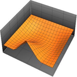
In[4]:=
ufun = NDSolveValue[{eqn, ic, bc}, u, {t, 0, 2}, {x, 0, 1},
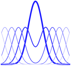
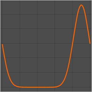
Method -> {"MethodOfLines"}];Visualize the periodic wavefunction.
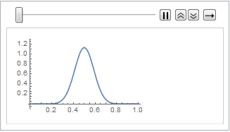
In[5]:=
plots = Table[
   Plot[ufun[t, x], {x, 0, 1}, PlotRange -> {-0.1, 1.3}], {t, 0,
    2, .1}];
ListAnimate[plots]