2015年のシカゴマラソンについて計算する

2015年10月11日に開催された2015年シカゴマラソンには45,000のランナーが集まった．37,000名以上のランナーが完走し，各ランナーのパフォーマンスの詳細は注意深く記録された．ここでは，このデータを含むカスタム実体ストアを使ってランナーとそのパフォーマンスの特徴を調べ，可視化する．

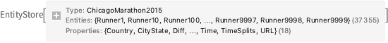
ResourceObjectからマラソンのEntityStoreをロードする．

In[1]:=

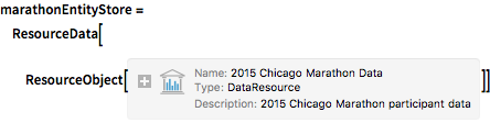
marathonEntityStore = ResourceData[ ResourceObject[ Association[ "Name" -> "2015 Chicago Marathon Data", "UUID" -> "7dc77972-cfc3-48dc-8d08-0292c6d2a929", "ResourceType" -> "DataResource", "Version" -> "1.0.0", "Description" -> "2015 Chicago Marathon participant data", "ContentSize" -> Quantity[1990.2215919999999`, "Megabytes"], "ContentElements" -> {"Content"}]]]

Out[1]=

このセッション用にストアを登録する．

In[2]:=

PrependTo[$EntityStores, marathonEntityStore];

ランナー総数と，隠的に定義された実体クラスを使って，男性の人数と女性の人数を取り出す．

In[3]:=

EntityValue["ChicagoMarathon2015", "EntityCount"]

Out[3]=

In[4]:=

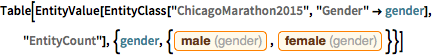
Table[EntityValue[ EntityClass["ChicagoMarathon2015", "Gender" -> gender], "EntityCount"], {gender, {Entity["Gender", "Male"], Entity["Gender", "Female"]}}]

Out[4]=

5人のランナーをランダムに選ぶ．

In[5]:=

RandomEntity["ChicagoMarathon2015", 5]

Out[5]=

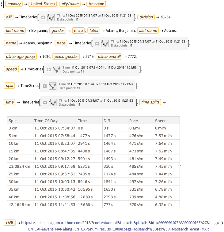
特定のランナーについて保存された特性を見る．

In[6]:=

Entity["ChicagoMarathon2015", "Runner145"]["PropertyAssociation"]

Out[6]=

ランナーの国籍の合計を抽出し，参加ランナーが多かった諸国の表を作る．

In[7]:=

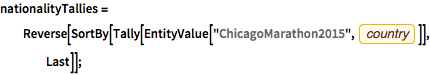
nationalityTallies = Reverse[SortBy[ Tally[EntityValue["ChicagoMarathon2015", EntityProperty["ChicagoMarathon2015", "Country"]]], Last]];

In[8]:=

TextGrid[Join @@@ Transpose[ Partition[Take[Reverse[Sort[Reverse /@ nationalityTallies]], 80], 20]], Alignment -> {{{Decimal, Left}}, Automatic}, Dividers -> {{{Thick, True}}, {{True}}}, Frame -> Thick, Background -> {Automatic, {{LightBlue, None}}}] // TraditionalForm

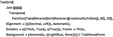
Out[8]//TraditionalForm=

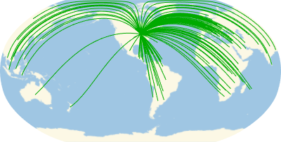
ランナーの全出身国からシカゴまでの測地経路を可視化する．

In[9]:=

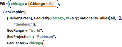
With[{chicago = Entity["City", {"Chicago", "Illinois", "UnitedStates"}]}, GeoGraphics[{Darker[Green], GeoPath[{chicago, #} & /@ nationalityTallies[[All, 1]], "Geodesic"]}, GeoRange -> "World", GeoProjection -> "Robinson", GeoCenter -> chicago]]

Out[9]=

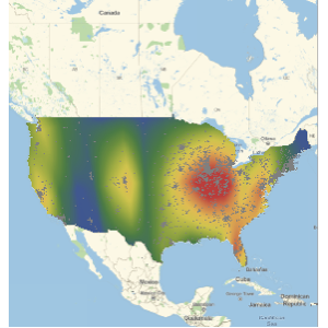
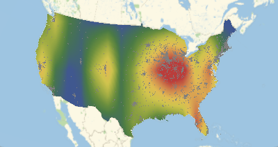
アメリカ国籍の参加者の出身地を示す合衆国のヒートマップを作る．

In[10]:=

anyUS = EntityClass["ChicagoMarathon2015", "Country" -> Entity["Country", "UnitedStates"]] // EntityList;

In[11]:=

allUSCities = DeleteMissing[ EntityValue[anyUS, EntityProperty["ChicagoMarathon2015", "CityState"]]]; talliedUSCities = Tally[allUSCities]; coordsUS = EntityValue[talliedUSCities[[All, 1]], "Position"]; cityPositions = Transpose[{coordsUS, talliedUSCities[[All, -1]]^0.5}]; projectionUS = {"LambertAzimuthal", "Centering" -> GeoPosition[{37.1558, -95.883}]}; data = {GeoGridPosition[#1, projectionUS][[1]], #2} & @@@ cityPositions; weightedData = WeightedData @@ Transpose[data]; cityDensityP = SmoothKernelDistribution[weightedData, "Silverman"]; cityDensity[{lat_Real, lon_Real}] := With[{xy = First[GeoGridPosition[GeoPosition[{lat, lon}], projectionUS]]}, Flatten[{xy, PDF[cityDensityP, xy]}]]; area = GeoVariant[Entity["Country", "UnitedStates"], "DefaultMapArea"]; {{latminUS, latmaxUS}, {lonminUS, lonmaxUS}} = GeoBounds[area];

In[11]:=

cityPlot = ContourPlot[ Sqrt[Last[cityDensity[{lat, lon}]]], {lon, lonminUS, lonmaxUS}, {lat, latminUS, latmaxUS}, Frame -> False, PlotRange -> All, Contours -> 100, MaxRecursion -> 2, ColorFunction -> ColorData["DarkRainbow"], PlotRangePadding -> 0, ContourStyle -> None];

In[11]:=

GeoGraphics[{GeoStyling[{"GeoImage", cityPlot}], Polygon[area], Gray, Opacity[1], PointSize[0.001], Point[coordsUS]}, GeoRange -> area]

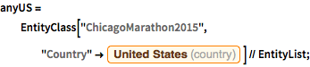
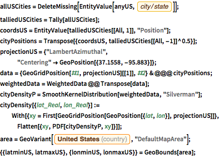
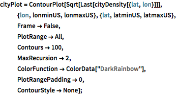
Out[12]=

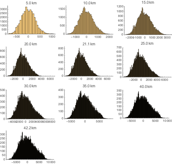
区間平均から差異ごとにランナー数を求める．

In[13]:=

allkm = Table[ Normal[allTimeSplits[[i]][2 ;;, "Time"]], {i, Length[allTimeSplits]}];

In[13]:=

allsplitbins = DeleteMissing[Transpose[allkm], 2];

In[13]:=

meanall = Table[N[Mean[allsplitbins[[i]]]], {i, Length[allsplitbins]}]

Out[13]=

In[13]:=

marathondistances = (allTimeSplits[[1]])[All, "Split"] // Normal

Out[13]=

In[13]:=

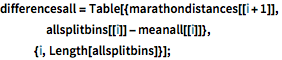
differencesall = Table[{marathondistances[[i + 1]], allsplitbins[[i]] - meanall[[i]]}, {i, Length[allsplitbins]}];

In[13]:=

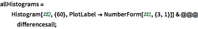
allHistograms = Histogram[#2, {60}, PlotLabel -> NumberForm[#1, {3, 1}]] & @@@ differencesall;

各区間についてのヒストグラムを生成する．

In[14]:=

Grid[Partition[allHistograms, UpTo[3]]]

Out[15]=

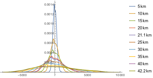
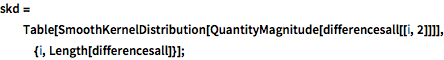
ランナーが区間を走った時間と平均時間の差の平滑化カーネル分布をプロットする．

In[16]:=

skd = Table[ SmoothKernelDistribution[ QuantityMagnitude[differencesall[[i, 2]]]], {i, Length[differencesall]}];

In[17]:=

Plot[ Evaluate[Table[PDF[skd[[i]], t], {i, Length[skd]}]], {t, -8000, 10000}, PlotRange -> All, PlotLegends -> Table[If[IntegerQ[QuantityMagnitude[diff = differencesall[[i, 1]]]], diff, Round[diff, .1]], {i, Length[differencesall]}] ]

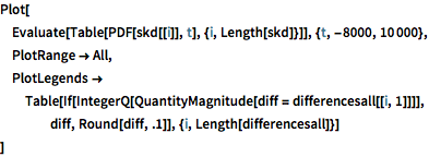
Out[17]=