Wolfram Language

Richer Knowledgebase Access

Running the Numbers on the 2015 Chicago Marathon

The 2015 Chicago Marathon drew 45,000 runners to Chicago on October 11, 2015. More than 37,000 completed the race, and details of each runner's performance were carefully recorded. Explore and visualize characteristics of the runners and their performances using a custom entity store containing this data.

Load an entity store of the marathon from a ResourceObject.

In[1]:=
Click for copyable input
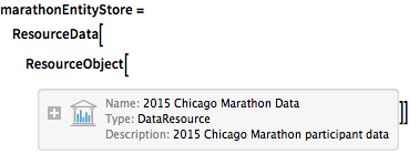
marathonEntityStore = ResourceData[ ResourceObject[ Association[ "Name" -> "2015 Chicago Marathon Data", "UUID" -> "7dc77972-cfc3-48dc-8d08-0292c6d2a929", "ResourceType" -> "DataResource", "Version" -> "1.0.0", "Description" -> "2015 Chicago Marathon participant data", "ContentSize" -> Quantity[1990.2215919999999`, "Megabytes"], "ContentElements" -> {"Content"}]]]
Out[1]=

Register the store for this session.

In[2]:=
Click for copyable input
PrependTo[$EntityStores, marathonEntityStore];

Extract the total numbers of runners and, using an implicitly defined entity class, the numbers of male and female participants.

In[3]:=
Click for copyable input
EntityValue["ChicagoMarathon2015", "EntityCount"]
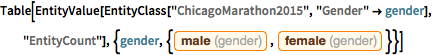
Out[3]=
In[4]:=
Click for copyable input
Table[EntityValue[ EntityClass["ChicagoMarathon2015", "Gender" -> gender], "EntityCount"], {gender, {Entity["Gender", "Male"], Entity["Gender", "Female"]}}]
Out[4]=

Select five random runners.

In[5]:=
Click for copyable input
RandomEntity["ChicagoMarathon2015", 5]
Out[5]=

View stored properties for a particular runner.

In[6]:=
Click for copyable input
Entity["ChicagoMarathon2015", "Runner145"]["PropertyAssociation"]
Out[6]=

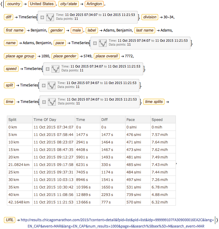
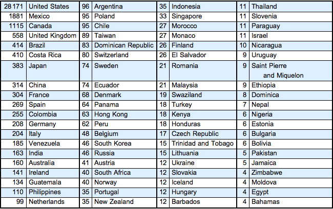
Extract tallies of runner nationalities and make a table of the most common nationalities.

In[7]:=
Click for copyable input
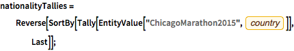
nationalityTallies = Reverse[SortBy[ Tally[EntityValue["ChicagoMarathon2015", EntityProperty["ChicagoMarathon2015", "Country"]]], Last]];
show complete Wolfram Language input
In[8]:=
Click for copyable input
TextGrid[Join @@@ Transpose[ Partition[Take[Reverse[Sort[Reverse /@ nationalityTallies]], 80], 20]], Alignment -> {{{Decimal, Left}}, Automatic}, Dividers -> {{{Thick, True}}, {{True}}}, Frame -> Thick, Background -> {Automatic, {{LightBlue, None}}}] // TraditionalForm
Out[8]//TraditionalForm=

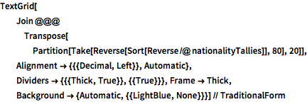
Visualize geodesic paths from all countries of origin to Chicago.
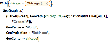
In[9]:=
Click for copyable input
With[{chicago = Entity["City", {"Chicago", "Illinois", "UnitedStates"}]}, GeoGraphics[{Darker[Green], GeoPath[{chicago, #} & /@ nationalityTallies[[All, 1]], "Geodesic"]}, GeoRange -> "World", GeoProjection -> "Robinson", GeoCenter -> chicago]]
Out[9]=

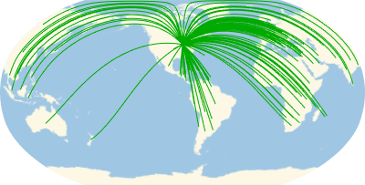
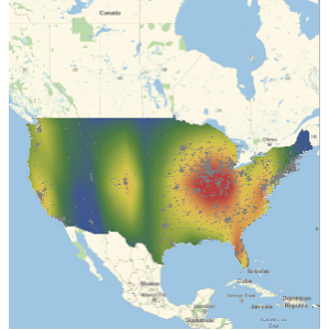
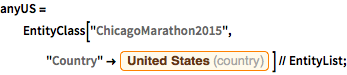
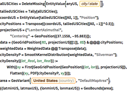
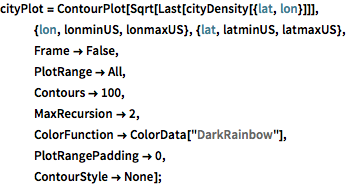
Construct a heat map of the US showing home locations for American participants.

show complete Wolfram Language input
In[10]:=
Click for copyable input
anyUS = EntityClass["ChicagoMarathon2015", "Country" -> Entity["Country", "UnitedStates"]] // EntityList;
In[11]:=
Click for copyable input
allUSCities = DeleteMissing[ EntityValue[anyUS, EntityProperty["ChicagoMarathon2015", "CityState"]]]; talliedUSCities = Tally[allUSCities]; coordsUS = EntityValue[talliedUSCities[[All, 1]], "Position"]; cityPositions = Transpose[{coordsUS, talliedUSCities[[All, -1]]^0.5}]; projectionUS = {"LambertAzimuthal", "Centering" -> GeoPosition[{37.1558, -95.883}]}; data = {GeoGridPosition[#1, projectionUS][[1]], #2} & @@@ cityPositions; weightedData = WeightedData @@ Transpose[data]; cityDensityP = SmoothKernelDistribution[weightedData, "Silverman"]; cityDensity[{lat_Real, lon_Real}] := With[{xy = First[GeoGridPosition[GeoPosition[{lat, lon}], projectionUS]]}, Flatten[{xy, PDF[cityDensityP, xy]}]]; area = GeoVariant[Entity["Country", "UnitedStates"], "DefaultMapArea"]; {{latminUS, latmaxUS}, {lonminUS, lonmaxUS}} = GeoBounds[area];
In[11]:=
Click for copyable input
cityPlot = ContourPlot[ Sqrt[Last[cityDensity[{lat, lon}]]], {lon, lonminUS, lonmaxUS}, {lat, latminUS, latmaxUS}, Frame -> False, PlotRange -> All, Contours -> 100, MaxRecursion -> 2, ColorFunction -> ColorData["DarkRainbow"], PlotRangePadding -> 0, ContourStyle -> None];
In[11]:=
Click for copyable input
GeoGraphics[{GeoStyling[{"GeoImage", cityPlot}], Polygon[area], Gray, Opacity[1], PointSize[0.001], Point[coordsUS]}, GeoRange -> area]
Out[12]=

Find the numbers of runners per variation from split mean.

In[13]:=
Click for copyable input
allkm = Table[ Normal[allTimeSplits[[i]][2 ;;, "Time"]], {i, Length[allTimeSplits]}];
In[13]:=
Click for copyable input
allsplitbins = DeleteMissing[Transpose[allkm], 2];
In[13]:=
Click for copyable input
meanall = Table[N[Mean[allsplitbins[[i]]]], {i, Length[allsplitbins]}]
Out[13]=
In[13]:=
Click for copyable input
marathondistances = (allTimeSplits[[1]])[All, "Split"] // Normal
Out[13]=
In[13]:=
Click for copyable input
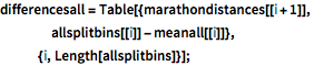
differencesall = Table[{marathondistances[[i + 1]], allsplitbins[[i]] - meanall[[i]]}, {i, Length[allsplitbins]}];
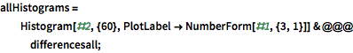
In[13]:=
Click for copyable input
allHistograms = Histogram[#2, {60}, PlotLabel -> NumberForm[#1, {3, 1}]] & @@@
 differencesall;

Generate histograms for each split.

In[14]:=
Click for copyable input
Grid[Partition[allHistograms, UpTo[3]]]
Out[15]=

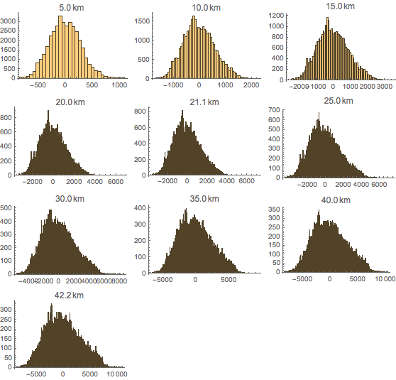
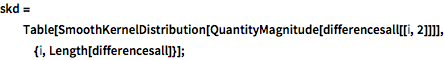
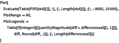
Plot a smooth kernel distribution of the differences between runners' splits and means.

show complete Wolfram Language input
In[16]:=
Click for copyable input
skd = Table[ SmoothKernelDistribution[ QuantityMagnitude[differencesall[[i, 2]]]], {i, Length[differencesall]}];
In[17]:=
Click for copyable input
Plot[ Evaluate[Table[PDF[skd[[i]], t], {i, Length[skd]}]], {t, -8000, 10000}, PlotRange -> All, PlotLegends -> Table[If[IntegerQ[QuantityMagnitude[diff = differencesall[[i, 1]]]], diff, Round[diff, .1]], {i, Length[differencesall]}] ]
Out[17]=

Related Examples

de es fr ja ko pt-br ru zh