球体メルカトルと楕円体メルカトル

メルカトル図法では，地球を表すのに球体モデルを使うか楕円体モデルを使うかによって結果が異なる．Wolfram言語では，どちらの場合も使える．

ほとんどの地図Webサーバで使われる投影法では，地球の球体モデルが使われており，これは通常「Webメルカトル」と呼ばれる．

In[1]:=

webMercator = {"Mercator", "ReferenceModel" -> GeodesyData["WGS84", "SemimajorAxis"]}

Out[1]=

In[2]:=

ellipMercator = {"Mercator", "ReferenceModel" -> "WGS84"}

Out[2]=

両方の図法を使って，オックスフォード大学の位置を変換する．

In[3]:=

p = GeoPosition[ Entity["University", "UniversityOfOxfordUnitedKingdom36022"]]

Out[3]=

In[4]:=

GeoGridPosition[p, webMercator][[1]]

Out[4]=

In[5]:=

GeoGridPosition[p, ellipMercator][[1]]

Out[5]=

北座標では33kmを越える違いがある．

In[6]:=

GeoGridPosition[p, webMercator][[1]]; GeoGridPosition[p, ellipMercator][[1]]; %% - %

Out[6]=

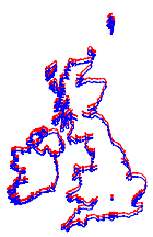
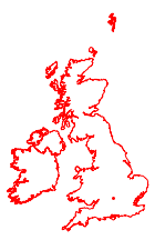
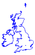
両方の投影法を使って英国とアイルランドの地図をそれぞれ描画すると，どちらの場合もほぼ同じに見える．

In[7]:=

webmap = GeoGraphics[{FaceForm[], EdgeForm[Red], Polygon[{Entity["Country", "UnitedKingdom"], Entity["Country", "Ireland"]}], Red, Point[p]}, GeoProjection -> webMercator, GeoBackground -> None][[1]]

Out[7]=

In[8]:=

ellipmap = GeoGraphics[{FaceForm[], EdgeForm[Blue], Polygon[{Entity["Country", "UnitedKingdom"], Entity["Country", "Ireland"]}], Blue, Point[p]}, GeoProjection -> ellipMercator, GeoBackground -> None][[1]]

Out[8]=

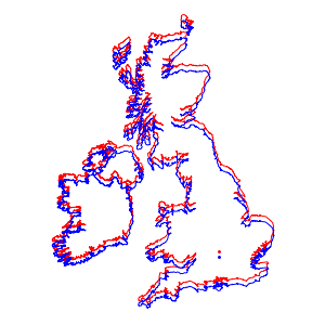
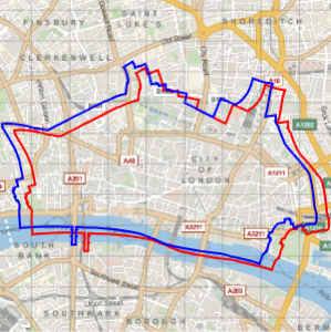
ところが，同一の地図上に置いてみるとその差がはっきりと分かる．

In[9]:=

Show[webmap, ellipmap]

Out[9]=