Trajectory Optimization
Minimize  subject to
  .
.
This example demonstrates how a variational problem can be discretized to a finite optimization problem efficiently solved by convex methods, such as QuadraticOptimization.
The variational problem will be approximated by discretizing the boundary value problem and using the trapezoidal rule to integrate on a uniformly spaced grid on the interval [0,1],  with
with  .
.
Let the variable u[i] represent  and x[i] represent
  for
for  .
.
The differential equation constraint is easily represented using centered second-order difference approximations for  from 1 to
  .
.
At the boundary, the zero derivative conditions allow for the use of fictitious points  and
and  . When
  and
and  , the second-order difference formula for the first derivative
 is zero for
  and
and  . Thus, at the boundary, use the following.
The trapezoidal rule for  is given by the following.
Since the expression from the trapezoidal rule is quadratic and all of the constraints are linear equality constraints, the minimum of the discretized integral can be found using QuadraticOptimization directly.
Approximate functions are constructed with Interpolation.
An exact analytic solution,  , is known for this problem, so it is possible to plot the error in the discretization.
The asymptotic error is roughly  , so by doubling
  to 200 and recomputing, the error will be about 1/4 of what is shown here.
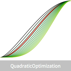
The analytic solution can be found by considering a family of curves  where
where  is a parameter. This parametric curve satisfies the prescribed boundary conditions
  . Since
  , one can find an optimal parameter
  that minimizes
  .
.
The optimal value of  is at 2, which is the analytic result
  .
.
