In Chapter 5, How It Works, we saw what machine learning models are and how they can learn. Let’s dive further into this topic by introducing the classic machine learning methods that are used for classification and regression. Some of these methods are about as old as computers themselves (e.g. nearest neighbors or decision trees), and the most advanced ones were developed in the 1990s (e.g. random forest, support-vector machine, or gradient boosted trees). All of these methods can be considered “off the shelf” since they are easy to use and available in most machine learning libraries. These methods are also general purpose, which means that they are not specialized for a particular kind of data. In practice, these methods are heavily used on structured data (such as spreadsheets with numbers and categories) but less on unstructured data (such as text, images, or audio), for which neural networks are often better (see Chapter 11, Deep Learning Methods). Usually, these methods are used in conjunction with feature engineering, which means obtaining good features “by hand” (see Chapter 9, Data Preprocessing).
This chapter will cover what these classic methods are, how they work, and what their strengths and weaknesses are. Understanding how these methods work is not absolutely necessary to practice machine learning, but it can be helpful for building better models and when automatic tools are not available.
Illustrative Examples
First, let’s define a few datasets that we will use to illustrate these methods. These simple datasets are not really meant to represent real-world data; they are only used to visualize and understand the models produced by these methods.
For classification, we will use the classic Fisher’s Irises dataset for which we drop the petal length and petal width and add a bit of noise to remove duplicate examples for visualization purposes:
Let’s also remove the units to simplify the preprocessing:
Here is the resulting dataset:
From this dataset, we will learn how to classify the species of irises as function of their sepal length and width.
For regression, we will use the Boston Homes dataset, for which the goal is to predict the median price of houses in a suburb as function of the suburb characteristics. Again, we keep only two features for visualization (the average number of rooms and the average age of the houses):
Here is was this dataset looks like:
Linear Regression
Let’s start with the oldest and simplest method, called linear regression, which is a parametric method used for regression tasks. This method originated in the beginning of the nineteenth century for fitting simple datasets (without computers at the time…). Linear regression has since been adopted for statistics and machine learning applications. Despite its simplicity, this method can be effective, and it is one of the most common methods used in the industry to handle structured data.
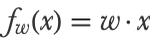
We already had a glimpse at what linear regression is in Chapter 5, How It Works, when parametric models were introduced. Let’s now look at a more complete definition in machine learning terms. The basic idea of linear regression is to predict a numeric variable using a linear combination of numeric features:

Here x1, x2, etc. are the features and w1, w2, etc. are the numeric parameters (called weights in neural network terms) that define the model f. This model can also be written more simply as a dot product between the feature vector x={x1,x2,...} and the vector of parameters w={w1,w2,...}:
For example, if x={1,2,3} and w={4,5,6}, the model would predict 32:
If there is only one feature, the model is a simple line, but if there are more features, it is a plane or hyperplane.
Linear regression should not be seen as just fitting a plane on the raw data though. Indeed, one can create many features from the data in order to obtain more complex models. For example, curve fitting with a polynomial is actually a linear regression in disguise for which the features are x={1,u,u2,...}, where u is the unique input variable:
In the four-dimensional space of features, the model is linear, but in the original space, it is a polynomial curve. Note that we included a constant feature here, x1=1, in order to create a nonzero prediction when all features are zero, which is a typical thing to do. The corresponding weight (which is also the prediction value at the origin) is called an intercept in statistical terms or a bias in neural network terms.
This feature engineering part is the key to creating powerful models using the linear regression method (and, more generally, for any classic machine learning method). It requires the understanding of the problem at hand and knowing a little bit about how this method works. Note that all features must be numeric here, so any other kind of feature has to be preprocessed into numeric values.
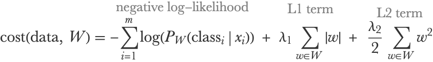
Linear regression models are trained by optimizing a cost function that is generally the total squared error plus some regularization terms. If we have n features and m examples and xi and yi are the input and output of example i, the cost function can be written as follows:
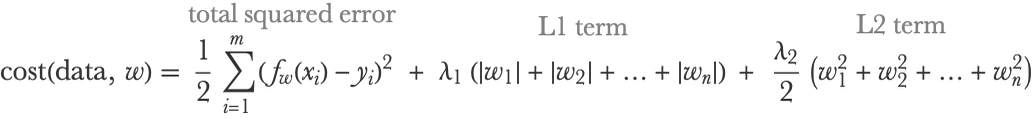
λ2 is a hyperparameter controlling the strength of the L2 regularization term, which helps generalization by shrinking the parameters w toward zero (but never exactly zero). Similarly, λ1 is a hyperparameter controlling the L1 regularization term, which shrinks parameters toward zero as well (and sometimes exactly zero, a property that can be utilized for discarding non-important features). Note that features and outputs have to be standardized, or at least centered, for this regularization to make sense. We can see that if the number of examples is large (large m), the regularization terms will not have a great influence, as expected. One nice thing about this cost function is that it is convex, so it is pretty easy to find its minimum. Even better: there is a closed-form formula to find its minimum exactly and efficiently using linear algebra.
Let’s fit a linear regression on our data and specify values for the two regularization hyperparameters:
Let’s now visualize the predictions:
As expected, the predictions form a plane that more or less captures the data. Note that if we had not defined values for the regularization coefficients, they would have been determined automatically through an internal cross-validation.
While linear regression can be set up as a non-probabilistic model (i.e. just returning a prediction), it can also be probabilistic. This is usually done by wrapping a normal distribution around the prediction. The predictive distribution of the output y for a given input x is then:
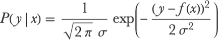
Here σ is the standard deviation of the distribution, which can be seen as the noise in the data (deviations that cannot be predicted). It is possible to learn a linear regression model by directly maximizing the likelihood using this distribution. As it happens, this maximum likelihood estimation is strictly equivalent to minimizing the mean squared error cost and then computing σ as the root mean square of the residuals. The regularizing coefficients λ1 and λ2 can also have a probabilistic interpretation. For example, setting a specific value for λ2 is equivalent to setting a Gaussian prior over the parameters w in a Bayesian learning setting and using a maximum a posteriori estimate (see Chapter 12, Bayesian Inference). Similarly, λ1 corresponds to a Laplace distribution prior.
We can extend and modify the linear regression method in many ways, such as using other loss functions, using a different predictive distribution, or even having the noise σ depending on the input value, but the definition presented here is the most common.
While old and simple, linear regression is still a very useful machine learning method: it is easy and fast to train, it can be used on large datasets, and the resulting model is small and fast to evaluate. Another advantage of this simplicity is that it is easy to deploy a linear regression model anywhere. Finally, the model is easily interpretable. For example, a large weight means that the corresponding feature is important for the model (if the data is standardized), and this is why this method is used a lot in statistics. Also, for a given prediction, we can directly look at the contribution wjxj of a given feature j to see the role played by this feature.
On the downside, the linear regression method does not generally perform as well as more advanced methods such as ensemble of trees. Also, the linear regression method typically requires more work from us to find the right features than these advanced methods. Finally, linear regression is particularly “shallow,” which means it is not so appropriate for solving perception and similar problems from scratch (neural networks are by far the best solution for these problems).
Overall, the linear regression method is still a popular solution in industrial settings to tackle structured-data problems, especially when simplicity or explainability is required. This method is also always useful as a baseline.
Logistic Regression
The logistic regression method is a simple parametric method, which is the equivalent of the linear regression method but for classification problems. (In machine learning terms, “regression” is a bit of a misnomer here since it is used to predict a class and not a numeric variable. This name comes from statistics, for which “regression” is more generic.) This method has many other names, such as logit regression, softmax regression, or even maximum entropy classifier (MaxEnt). Like linear regression, the logistic regression method is simple, can be effective, and is often used in the industry to tackle structured data problems.
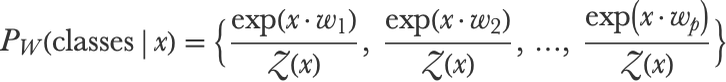
Let’s directly define the logistic regression method for an arbitrary number of classes, which is sometimes called a multinomial logistic regression (see Chapter 5, How It Works, and the Support-Vector Machine section of this chapter for a specific analysis of the binary case). Logistic regression returns a probabilistic classifier, which means that we have to compute a probability for each possible class given an example x. This can be represented by a probability vector:

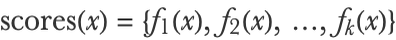
This vector also represents a categorical distribution over the possible p classes. The first step to obtain these probabilities is to compute a score for each class using linear combinations of features:

Here x is a vector of numeric features, and each wk is a numeric vector (not just a number this time) of parameters corresponding to a given class k. Each score x·wk is a dot product between these two vectors, like in a linear regression (and we could add a bias term, or just use x1=1 as we explained in the previous section). If there are n features in the vector x, this means that there are pn parameters in total, which we can represent by a matrix W of size pn. As an example, let’s say that W is the following 32 matrix:
This means that there are three classes and two features. Let’s now say that the feature vector x for a given example is as follows:
We can then compute the scores using a matrix-vector product (which is equivalent to the p dot products defined earlier):
Now we need to transform these scores into a proper categorical distribution, which means that the probabilities need to be non-negative and sum to 1. This is done using the softmax function, also called LogSumExp, which is a multivariate version of the logistic function (from which this method is named). The first step of the softmax function is to compute the exponential of every score:

In our example, this gives:
All scores are now positive by construction. The second step of the softmax is to normalize these scores. We can do this by first summing the scores to compute a normalization constant (called a partition function for historical reasons):

So in our example, this gives:
Then we just need to divide the scores by this normalization term to obtain our final probability vector:
Going back to our example, we have:
As we can see in our example, the probabilities obtained are positive and sum to 1, so they form a valid categorical distribution. A program for this model could simply be:
Which on our example gives:
We could also implement this model as a neural network (see Chapter 11, Deep Learning Methods):
This model gives the same result as before:
As you can see, logistic regression is just a linear transformation with a bit of post-processing to return probabilities. The scores before the softmax function are often called the logits and can be seen as unnormalized log-probabilities.
As for linear regression, the typical way to train a logistic regression is by minimizing a cost function, which in this case is the negative log-likelihood (see Chapter 3, Classification) plus some regularization terms. If we have m examples and xi and classi are the feature vector and class of example i, the cost function can be written as follows:
The negative log-likelihood term pushes the model to give high probabilities to correct classes (classi), while the regularization terms push weights to be small to ensure generalization. These L1 and L2 regularization terms are the same as in the linear regression case; the only difference is that they are sums over the elements of a matrix instead of a vector. Programmatically, we would write them as follows:
Unlike the linear regression case, there is no simple closed-form solution to find the minimum of this cost, so we have to perform an optimization procedure. Fortunately, this cost function is convex, so the optimization is easy and reasonably fast compared to other machine learning methods.
Let’s now apply the logistic regression method on our toy dataset, without any regularization, and visualize the decision regions:
We can see that the resulting model separates the space into three contiguous regions, and that the boundaries are lines because logistic models are linear classifiers. If we needed this method to produce nonlinear boundaries, we would need to add extra features, like we did in the linear regression example. We can see that some training examples are misclassified, which is not necessarily a bad thing (see Chapter 5, How It Works). Let’s now visualize the probabilities predicted by the classifier.
We can see smooth surfaces with logistic-sigmoid shapes at the boundaries and also a sharp transition near the setosa boundary. This sharp transition makes sense because the setosa training examples can be perfectly separated with this linear classifier and we did not set any regularization. If we set a higher L2 regularization value, for example, the transitions are smoother:
Note that the classification regions have been modified as well by this regularization. The regularization strength should be properly tuned using a validation procedure or by letting high-level tools such as Classify do the job automatically.
The logistic regression method shares the same strengths and weaknesses as the linear regression method. On the upside, it is simple, fast, small in memory, and easy to export. On the downside, it requires more feature engineering than others, is generally beaten by ensemble of trees in terms of classification quality, and is not suited for perception problems.
Overall, the logistic regression method is still a popular solution in industrial settings to tackle structured-data problems and to obtain baseline models.
Nearest Neighbors
Nearest neighbors is the prototypical example of nonparametric methods and arguably the simplest and most intuitive machine learning method. One strength of this method is its versatility: it can be used for a variety of tasks, such as classification and regression, and for all kinds of data (as long as we can define a measure of similarity between examples). While naive, this method should not be ignored. It is sometimes sufficient to solve the problem at hand, and it is generally a useful baseline. In Chapter 5, we introduced this method and showed how it can be used to recognize handwritten digits. Let’s now expand on this introduction and define the nearest neighbors method more precisely.
The central idea of nearest neighbors is that examples that have similar features tend to have similar labels. This sort of continuity assumption is implicitly made by most machine learning methods, but in this case, it is explicit. Let’s start with the classification task and consider the simple case where we have a dataset of two numeric features, age and weight, and two possible classes, cat (![]() ) and dog (
) and dog (![]() ):
):
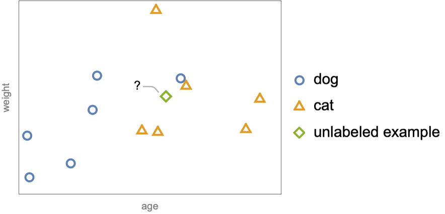
The example ![]() is unlabeled and we want to determine its class. Nearest neighbors does this by first identifying the “neighbors” of the unlabeled example. The neighbors can be defined as the examples inside a sphere of a given radius centered around the unlabeled example:
is unlabeled and we want to determine its class. Nearest neighbors does this by first identifying the “neighbors” of the unlabeled example. The neighbors can be defined as the examples inside a sphere of a given radius centered around the unlabeled example:
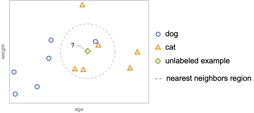
The next step is to choose the most frequent class amongst these neighbors. Here, the unlabeled example has three cat neighbors and only one dog neighbor, so the predicted class is cat. This simple procedure can also be adapted to the regression task. Let’s show this on a similar dataset for which labels are now numeric values, such as the speeds of the animals (represented by different colors):
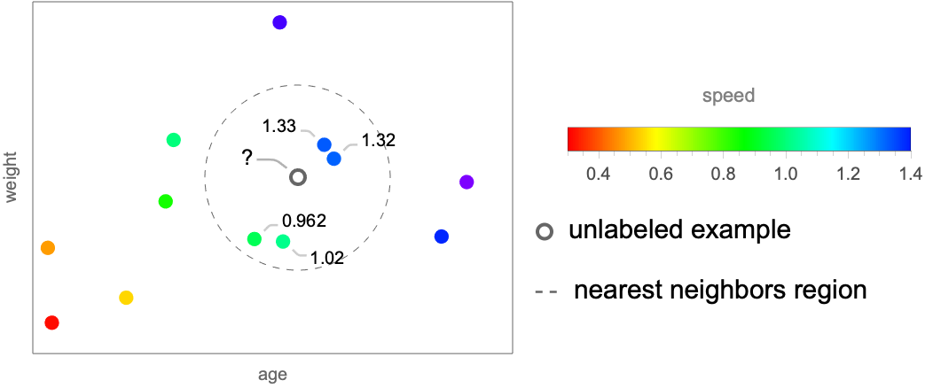
We can predict the speed of the unlabeled example![]() by averaging the speeds of the neighbors. In this case, this would give:
by averaging the speeds of the neighbors. In this case, this would give:
And that’s pretty much what the nearest neighbors method is. This method can be seen as a sort of moving average, or smoothing, which interpolates between the training data. You will notice that there is not really a learning procedure here (only hyperparameters can be learned) and that the resulting model has to store all the training data in order to make predictions.
There are several variations of this method. By far the most popular one uses a different way to define neighbors. Instead of using a fixed-size sphere, the neighbors are the k (a fixed number) nearest examples. This version is called k-nearest neighbors, abbreviated k-NN, and it generally works better than when using a fixed-size sphere (e.g. when the dataset shows a high variability in its example density). Another variant is to use all examples instead of just neighboring ones and weighting these examples according to how distant they are. Typically, one would use a similarity function, such as an exponential decay, to define these weights:
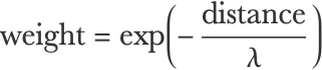
This similarity function assigns high weights to examples that are neighbors and low weights to distant examples. λ is a scaling constant that can be interpreted as a radius. Each prediction is then made by computing a weighted average over all examples. This is a smoother version of nearest neighbors, and it can be seen as a kernel method (see the Support-Vector Machine section in this chapter).
Regardless of the method variant, we always have to define a distance or dissimilarity function. This function depends on the data type. For example, we can use a Euclidean distance for numeric data:
For string data, we could use an edit distance:
We can imagine all sorts of variations to better adapt to a particular dataset (including combining distances when many types are present). When the data type is simple (e.g. a numeric vector), we can use one of the classic distances. When the data type is more complex (e.g. a dataset of social media profiles that contains text, pictures, and all sorts of other data types), we can get more creative and figure out a custom distance or dissimilarity function that fits our needs based on our knowledge of the data and the problem.
The final thing that we need to define is the size of the neighborhood. In the fixed-sphere version, this size is the radius of the sphere, and in the k-NN version, it is the value of k. The size of the neighborhood is a very important hyperparameter to consider because it allows for the control of the capacity of the model. For example, let’s train a k-NN classifier with k=1 on our toy dataset and visualize the decision regions:
We can see that the regions are fragmented and that the boundaries show a lot of variations, which makes sense since every example defines its own small prediction region around it. This setting of k=1 is certainly not the optimal value; we are probably overfitting. Let’s compare this with the decision regions when k=20:
The decision regions are now less fragmented. We reduced the fitting ability of the model, and, therefore, the model fits less noise than for k=1 (more model bias and less model variance). As for every other regularization parameter, the optimal value for k should be determined using a validation set or by cross-validation.
As presented here, the nearest neighbors method produces non-probabilistic models. It is, however, possible to obtain a predictive distribution by estimating the class distributions of neighbors. In our previous example, the neighbors were three cats and one dog, which would lead to the following probabilities:
Typically, we would smooth these probabilities, such as adding 1 to each class count (this is called an additive smoothing or Laplace smoothing):
Such smoothing allows for the avoidance of zero probabilities and usually improves the negative log-likelihood on a validation set. Again, the type and strength of smoothing can be determined through a validation procedure, which can lead to a decent probabilistic classifier. Let’s visualize the probabilities determined by our k=20 model:
As expected, these probabilities are less smooth than in the logistic regression case, which is typical of nonparametric methods.
Let’s now visualize the predictions of the nearest neighbors method on the housing dataset:
The predictions seem sensible and fairly smooth. Note that this is not a plane like in the linear regression case, which is why such methods are said to be nonlinear. The number of neighbors has been determined automatically here, which happens to be 20:
As we saw, nearest neighbors is not really learning anything; it is directly using the raw data in order to make predictions. This is sometimes called lazy learning. One advantage of this lazy learning is that the training phase is very fast. On the other hand, the resulting model is memory intensive since all training examples have to be stored. Also, making predictions can be slow if the dataset is large, even though there are a number of techniques to retrieve neighbors efficiently. All of these particularities have to be taken into consideration.
Naturally, the nearest neighbors method does not provide the best predictions out of the box. For example, this method cannot learn that some features are more important that others or that some training examples are more important than others. This means that in order for this method to work well, we generally have to create good features by hand or define a good distance function. Note that we only need a distance function to use this method, and this is a strength compared to other classic methods. When the data type is complex or unusual, it can be easier to come up with a reasonable distance or dissimilarity rather than figure out how to properly process the data into something like numeric vectors.
Overall, nearest neighbors is not the most used machine learning method, but it has its strengths and can be a useful baseline.
Decision Tree
The decision tree method is another classic nonparametric method that can be used for both classification and regression. Generally, this method does not provide great models in terms of predictions, but it is fast and the resulting models can (sometimes) be interpretable, which is needed for some applications. Also, this method is at the heart of much stronger methods using ensembles of decision trees called random forests and gradient boosted trees.
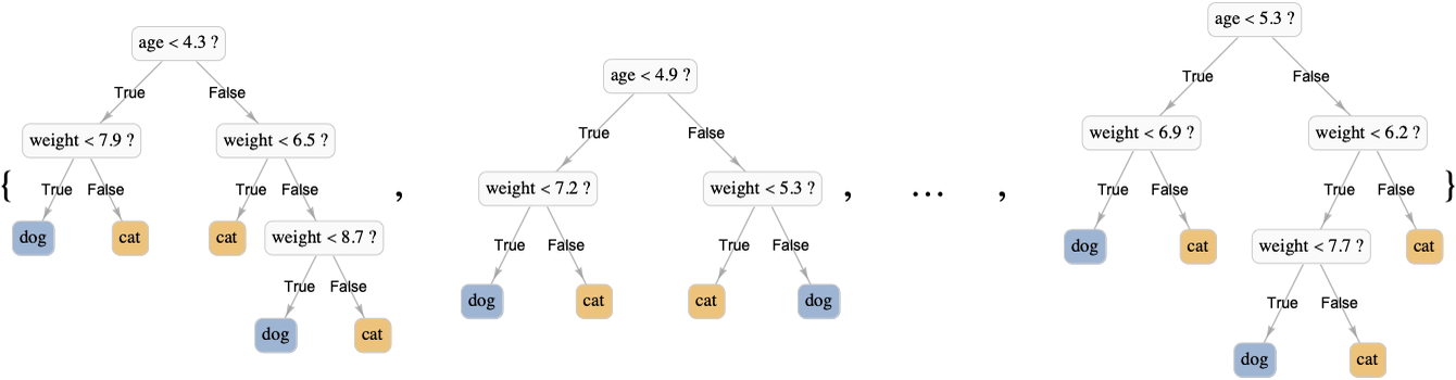
The goal of the decision tree method, as its name indicates, is to learn a decision tree from the data in order to make predictions. A decision tree is a model that figures out the label of a given example by asking a series of questions such as, “Is the feature "age" greater than 3.5 or not?” or “Is the feature "color" equal to blue or not?” It is a bit like in spoken games during which people try to guess a secret object by asking questions about it. The set of questions that can be asked are organized hierarchically in a tree structure. Here are examples of such trees for a classification and a regression task:
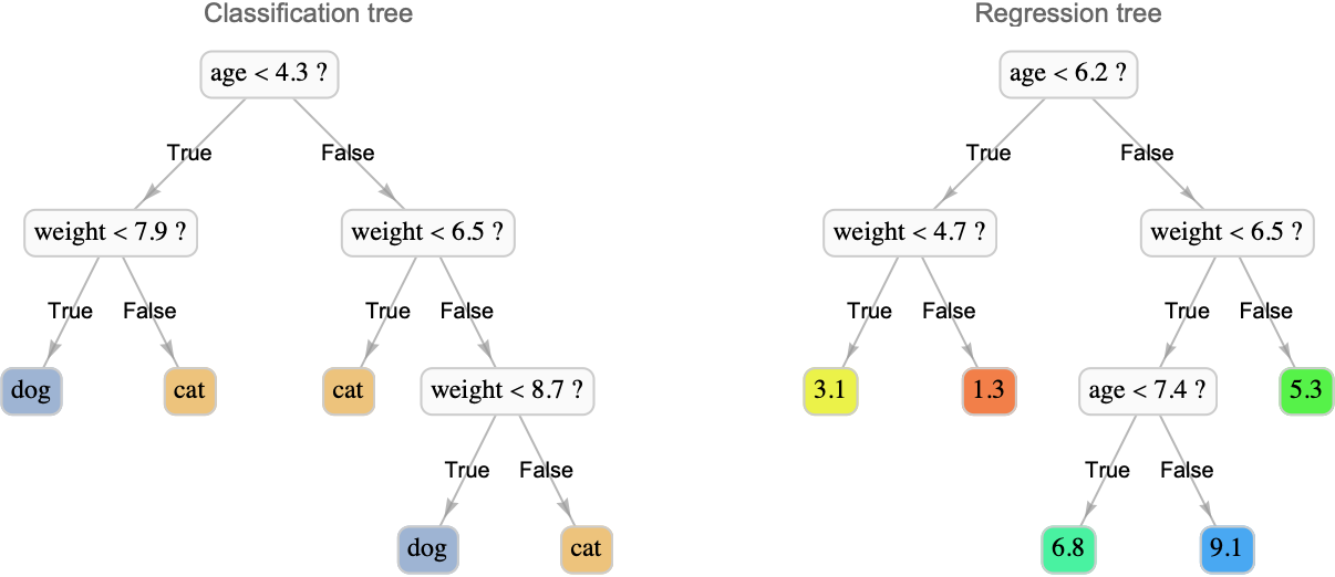
Each node is a question, which, in this case, can only be answered by true or false. In order to make a prediction, one should first answer the question at the root of the tree, which tells us which branch to go to: left if the answer is true and right otherwise. We then answer the next question and so on until we reach a leaf. Each leaf of the tree is a class or a label value, which corresponds to the prediction. Questions are generally simple in such trees, but this is not an issue. By combining several simple questions (i.e. making the tree deeper), one can construct arbitrarily complex decision functions. There is an incentive to keep trees small though because small trees are less prone to overfitting but also because they are more interpretable than big trees. For example, a domain expert could analyze a tree to see if the questions make sense or we could extract the few questions that led to a particular decision to help understand this decision. In some applications, this explainability is necessary. When trees are larger though, this interpretability is going away, so they can be considered black box models.
A decision tree can be seen as a hierarchical partitioning of the feature space. Here is a visualization of this partitioning for the trees shown previously:
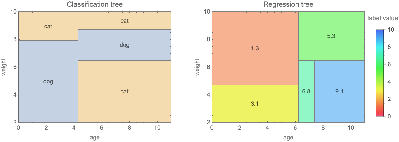
We can see that the space is partitioned into cells, which are rectangular because questions are about single features. Questions such as “age + weight < 5 ?” would result in slanted boundaries. The implicit assumption, like in nearest neighbors, is that similar examples should have similar labels. This model can be seen as a sort of nearest neighbors for which the neighborhoods are defined by fixed cells and not by a moving sphere or a number of neighbors. One key difference from the nearest neighbors method is that these boundaries are explicitly learned from the data.
Let’s now look at how such decision trees are trained. The goal is to obtain a partitioning that is able to make good predictions. The previous partitionings have been learned from the following training data:
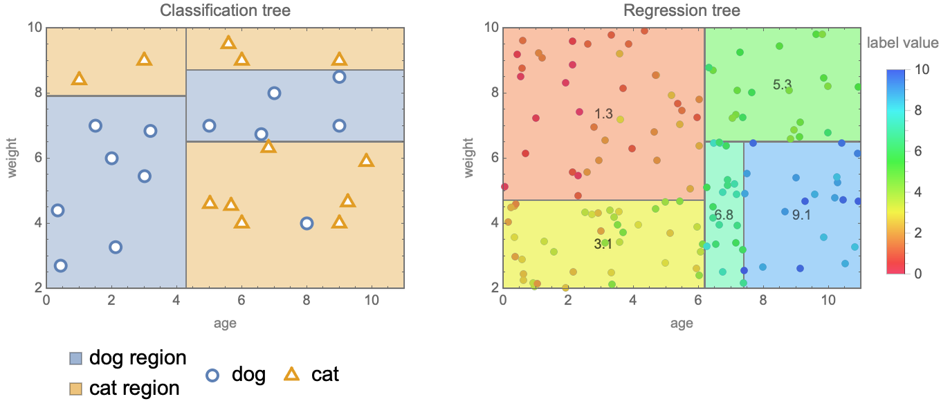
We can see that cells tend to contain examples having the same class or label value. This label separation is the first objective of the partitioning algorithm, which makes sense since the overall goal is to define regions belonging to a given class or value. A perfect class/value separation is not necessarily desired though because it could produce small cells that contain too few examples, which can lead to overfitting. To avoid this, the second objective of the partitioning algorithm is to obtain cells that are large enough or, similarly, to obtain trees that are not too deep. The partitioning algorithm tries to balance these two conflicting objectives in order to obtain a model with good prediction abilities.
The partitioning is typically performed in a top-down fashion, which means that the tree is grown from root to leaves. At first, the entire space constitutes a unique cell that includes all the training data. This mother cell is then split into two child cells according to a splitting criterion (mostly trying to separate classes/label values), and the training data is split according to these cells. At this point, the tree has only one node and two leaves/cells; it is called a stump. This process is then repeated for each child cell and again for descendant cells until some stopping criterion is reached, such as a minimum number of examples per cell or a maximum tree depth. An optional pruning procedure can also be performed to merge some cells. This simple, greedy algorithm works well in practice, and it is very fast so it can be used on large datasets. Here is what the prediction boundaries look like on our irises dataset:
The boundaries are rectangular as expected and quite simple in this case. It is generally possible to control the stopping criterion and the pruning in order to tune the complexity of the partitioning.
Like nearest neighbors, the decision tree method is not natively probabilistic. It is possible to obtain a predictive distribution by estimating the training label distribution in each cell, possibly with some smoothing involved. This is not ideal though, and such a model typically benefits from being calibrated (see the Classification Measures section of Chapter 3, Classification). Here are the class probabilities of our irises classifier:
We can clearly see the cells defined by the tree. Let’s now look at the predictions for the housing price problem:
As expected, the model fits the data with rectangular areas that have the same prediction value.
Decision trees are not providing the best predictions, but they are small, are fast to run, and can be interpretable. Interestingly, it is possible to keep the desirable properties of a classification tree while improving its prediction performance using a knowledge distillation procedure. The idea of knowledge distillation is to replace the labels of the training set with the class probabilities obtained from a good model and then train the decision tree on these “soft labels.” Such soft labels are more informative than hard labels, and they provide a powerful regularization that allows for the training of a simple model that generalizes well. Knowledge distillation is mostly used to reduce the size of neural networks, but it can also be used to obtain better decision trees.
Overall, the decision tree method is mostly used when interpretability is required but not so much otherwise. However, while decision trees do not provide great predictions by themselves, they can be combined to form the powerful random forest and gradient boosted trees methods, which are probably the best general-purpose machine learning methods.
Random Forest
Let’s now introduce one of the most popular generic machine learning methods, called random forest. Random forest is a nonparametric method based on decision trees and can, therefore, be used for both regression and classification. This method is fast to train, generally obtains good predictions and good predictive probabilities, and has the advantage of not requiring the tuning of hyperparameters, which makes it a great out-of-the-box method.
The model produced by random forest is an ensemble of decision trees (sometimes called a decision forest), which works by combining predictions of individual trees. Here is what such a forest could look like:
Each tree is trained independently on a random variation of the original dataset. These dataset variations are meant to be statistically similar to the original dataset but still different. One way to obtain such a variation is to use bootstrap samples of the dataset, which means sets of examples randomly sampled from the original dataset. Using bootstrap samples to train many models and averaging their results is called bagging (short for bootstrap aggregating). To understand this, let’s train an ensemble of decision trees on the irises dataset using the bagging procedure (not yet a proper random forest but almost). We first need to be able to resample the training set, which can be done using the RandomChoice function:
Here each example is independently chosen at random. Because this resampling can create duplicates, it is called a resampling with replacement. For each model of the ensemble, we need to resample the entire training set and learn a classifier on this new training set. Let’s create an ensemble of five trees:
Let’s now see how to make predictions with such an ensemble. We first need to compute the predictions of individual trees:
We can now combine these predictions by selecting the most common one:
We can also obtain probabilities by counting the predictions:
A better way to do this, though, is to average the probabilities given by the decision trees:
And that is how we can apply bagging to classification trees. For regression trees, the training procedure is the same except that we combine predictions by averaging them, such as:
We can also obtain a predictive distribution in this case by computing the standard deviation of these predictions:
An ensemble of bagged trees already constitutes a good machine learning method in terms of prediction abilities. Random forest improves this procedure further by adding a random feature selection. A given fraction of features, let’s say 40%, is randomly selected from the data and used to create a given node; the other 60% is dropped for this specific node. This typically improves the predictive performance of the ensemble further. Also, random forest grows trees almost fully and without pruning them. Let’s visualize the predictions of random forest for the irises classification problem:
We can recognize the vertical and horizontal boundaries inherited from the decision trees, but the boundaries are more complex this time. Let’s look at the probabilities given by this method:
We can see that the transitions are less abrupt than for a decision tree since we are averaging the results of many trees. Let’s now see what this method gives for the house pricing problem.
Again, the transitions are smoother, and seemingly better, than for a decision tree.
The random forest method typically obtains much better performance than the decision tree method that it is based on. One way to understand this is to see this “shaking and averaging” procedure that random forest does as a smart way to regularize decision trees. Indeed, fully grown trees (lots of leaves and only a few training examples per leaf) can learn complex patterns but are highly sensitive to the training data. If their training is unstable, two deep trees trained on slightly different datasets can end up being quite different. In statistical terms, this means that fully grown trees have a high variance and overfit the data because of this. The naive way to counteract this effect would be to reduce the size of the trees, but this would increase their biases and they would not be able to fit complex patterns anymore (they would be weak learners). This shaking and averaging procedure naturally causes the training to be stable since data variations are different for each tree and tend to cancel each other out when averaged. This has the effect of reducing the variance of the method and without adding much bias, which leads to a much better method overall. One thing to note is that the resulting model is not a tree anymore but an ensemble of trees, like for a model learned in a Bayesian way (see Chapter 12, Bayesian Inference).
This variance reduction without bias addition can appear too good to be true. One way to understand this is to see this shaking and averaging procedure as the addition of extra information to solve the problem, which can be formulated as “models that have been trained on similar datasets should give similar predictions.” Decision tree benefits a lot from this procedure, but this is not the case for all methods. For methods that are quite stable, such as nearest neighbors, this procedure is not worth it compared to other regularization strategies (e.g. increasing the number of neighbors). The training of neural networks, on the other hand, can be quite unstable, and in practice, a similar but much simpler procedure is used to enhance their performance: many models are trained from different initial weights in order to obtain an ensemble of networks that perform better when combined.
Random forest only has a few hyperparameters. The number of trees is one of them, but it is not a hyperparameter that gains from being tuned since adding trees cannot degrade the performance of the ensemble. In practice, having more than 1000 trees guarantees having just about optimal results (and fewer trees can be used to obtain a lighter and faster model). The depth of the trees is another possible hyperparameter, but it is not that useful either since we want fully grown trees. One hyperparameter that could gain from being tuned is the fraction of features that are selected for each node, even though library defaults generally give good performance. Overall, this method is quite hyperparameter free, which makes it appealing in terms of simplicity and training speed. Also, each tree is trained independently, which allows for the easy parallelization of the computation, which is something that gradient boosted trees cannot do.
Overall, the random forest method is a powerful general-purpose method that is fast to train and does not require hyperparameter tuning. Compared to simpler methods, it has the disadvantage that it can be large in memory and slow to make predictions if many trees are used.
Gradient Boosted Trees
The gradient boosted trees method is another method using an ensemble of decision trees to make predictions. This method can be used for both the regression and classification tasks, and it generally produces models that are as good or even better than random forest in terms of predictions. Gradient boosted trees is often considered the best general-purpose machine learning method for structured data, and it is a favorite with data scientists. The price to pay is that the training is slower than for random forest and that there are many hyperparameters to tune, making it more complex to handle.
Gradient boosted trees is based on the boosting procedure, which is a generic way of combining weak learners (methods that have a low capacity and thus cannot fit complex things) into a strong “boosted” learner. There are many variations of boosting, but the overall idea is to train many models sequentially (one after another) with each new model focusing on correcting the fitting errors of their predecessors, which is a rather intuitive idea.
Let’s use the most simple example of boosting on the housing price problem. We first start by training a linear regression on the data:
This tree does not perfectly fit the training data; the residuals of the model are nonzero:
A simple idea to obtain a better fit to the training data is to train another model on these residuals. Let’s do this using the nearest neighbors method:
We can now add the predictions of these two models to obtain a combined model with a better fit to the training data:
The residuals are now lower:
We could continue in this direction by training an additional model on the residuals of this combined model and so on to reduce the training errors further. However, while the fit on the training data is guaranteed to improve, we are not sure that the resulting model generalizes better, so we should stop adding models at some point in order not to overfit.
The gradient boosted trees method pushes this model-refinement idea to its limit by iteratively training up to thousands of small decision trees on the training data, each tree correcting the fitting errors of its predecessors by a little bit. Let’s create such an ensemble on the housing price data. As in our simple boosting example, each tree is trained to predict the residuals of the current ensemble and then added to the ensemble. One difference is that we weight each tree by a shrinkage factor v<1, which acts as a regularization hyperparameter. The final model is, therefore, a weighted sum of regression trees, which, for a given input x, can be written as:

And programmatically as:
Here is a program to train these trees:
Let’s train ensembles of two, five, and 20 trees with v=0.2 and visualize their predictions:
As expected, the fit improves as more trees are added. While the ensembles with two and five trees are not fitting the data very well (underestimating the data in this case), the ensemble with 20 trees starts to give a good fit. This is essentially what boosting does; it iteratively adds more models to refine the fit to the training data. As a consequence, even weak learners, such as small/shallow decision trees, can lead to a model that has a high capacity.
Increasing the capacity of a decision tree could also be done by growing the tree further, but it would increase its variance as well. As it happens, using such a boosting procedure works much better than simply using a larger tree. It is interesting to note that the philosophy of gradient boosted trees is the opposite of that of random forest. While random forest seeks to reduce the variance of large trees, gradient boosted trees seeks to reduce the bias of small trees. In a sense, one is a solution against overfitting and the other one is a solution against underfitting.
The boosting procedure that we described above can also be seen as a gradient descent in the space of predictive models. Indeed, each residual y-ypred (y is the true label and ypred is the prediction) is equal to the negative gradient of the mean squared loss function with respect to the prediction ypred:
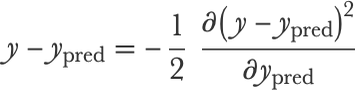
This means that a model trained on these residuals points toward an approximate steepest-descent “direction” (in model space) to minimize the mean squared loss. The whole procedure is a sort of gradient descent (see Chapter 11, Deep Learning Methods), which is where the name “gradient boosted trees” comes from. The shrinkage factor v can be interpreted as the learning rate of this gradient descent.
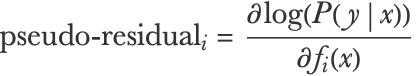
Following this gradient descent interpretation, gradient boosted trees can be adapted to minimize any differentiable loss function. For a model f, a training input x, and its corresponding training output y, we can compute the “pseudo-residual” as the negative gradient of the loss with respect to the prediction f(x):
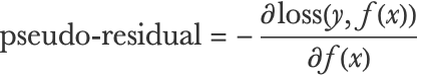
We can now just train a regression tree to fit these pseudo-residuals in order to update our ensemble and decrease the loss function.
The possibility of using any loss function (which is completely independent of the way the individual decision trees are trained) makes gradient boosted trees a very versatile method. In particular, we can train gradient boosted trees for classification problems. In the case of binary classification, we can train regression trees to predict a score function f(x) that will be used to define probabilities using the logistic function:

As usual, we want to minimize the negative log-likelihood, so if x is an input and y is its corresponding class, the pseudo-residual on which to train the regression trees would be:
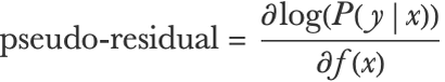
And this would give us a probabilistic binary classifier. Note that the trees here are regression trees and not classification trees. This can be generalized to the multiclass case by fitting k (one per class) ensembles of regression trees, each one predicting a function fi(x) representing the score for a particular class:
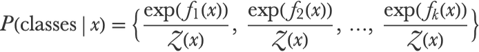
We can then transform these scores into probabilities with the softmax function (see the Logistic Regression section in this chapter):
During each boosting iteration, k new trees are therefore trained on the pseudo-residuals of the negative log-likelihood loss function:
And this procedure would give us a proper probabilistic multiclass classifier. Here are the classification regions of a gradient boosted trees classifier on our irises dataset:
Again, we recognize the vertical and horizontal boundaries inherited from the decision trees. Interestingly, the boundaries are less fragmented than in the random forest case, which is probably a good thing. Let’s look at the probabilities given by this method:
We can see the rectangular regions of decision trees, and the probabilities seem to show less variation than in the random forest case.
These are the basics of gradient boosted trees. There are many variants and improvements of this method. One of them is to resample the examples and features as random forest does. This allows for the merging of the methods of gradient boosted trees and random forest in order to obtain a better model. Another variant is to reweight the decision trees as a post-processing step (with a linear regression using tree predictions as features).
The gradient boosted trees method typically has a large number of hyperparameters to tune, sometimes more than 20. Tuning these hyperparameters can be a slow and daunting task and should generally be left to an automatic procedure, such as a random search or something more sophisticated (see the Hyperparameter Optimization section of Chapter 5, How It Works). The most important hyperparameters are related to the learning rate, the size of the trees, and the number of trees. The learning rate controls the speed at which the ensemble is converging toward a minimum cost, so it is tempting to give it a high value, but ensembles trained with a slow learning rate tend to generalize better, so values v<0.1 are typically chosen. The size of the trees directly affects the capacity of the model: trees with only one node (stump) only separate the space once while deeper trees can capture complex interactions between features, so a balance needs to be found. The number of trees is also important because, unlike in random forest, we can overfit by adding too many trees. One way to avoid this form of overfitting is by monitoring the cost function on a validation set as we add more trees and stopping the process when this cost goes up. This technique is known as early stopping and is principally used for neural networks (see the Regularization section of Chapter 5, How It Works).
Overall, gradient boosted trees is probably the best general-purpose method to tackle structured data problems and the most popular method to obtain good predictions. On the downside, it is slower and more complex to train than other classic methods (but still generally faster and simpler than neural networks) and the resulting model can be large.
Support‐Vector Machine
Let’s now introduce the support-vector machine (SVM) method, which was considered the best classification method in the late 90s and early 2000s (including for perception problems). Nowadays, deep learning methods are favored for perception problems, and ensemble of trees tends to be more used than SVM for structured data problems. Nevertheless, SVM is still an important method that is used for various machine learning applications.
SVM was originally a binary classification method that came in two different flavors: a linear parametric method and nonlinear nonparametric method. These two variants create very different kinds of models, but they are integrated into the same mathematical framework, which is why they are both SVMs. In a nutshell, the linear variant is a sort of logistic regression, and the nonlinear variant is a nearest neighbors that learns. Let’s describe them in more detail.
The first variant of SVM (and historically, the original one) is called linear SVM and produces a linear classifier. In a sense, linear SVM is a non-probabilistic version of the binary logistic regression (which is also a linear classifier). As in the binary logistic regression method, the class of an input x is determined by computing a linear combination of the features x={x1,x2,...}, which we can write as a dot product with a weight vector w={w1,w2,...}:
Here x and w are both numeric vectors. This value is then used to compute a score for each class:

For a given x, the class obtaining the highest score is chosen, which means that class A is chosen if w.x is positive and class B if it is negative. Here is an illustration of how two inputs, x and x′ would be classified for a given vector w:
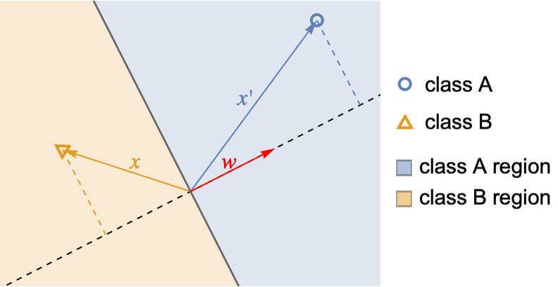
The decision boundary is defined by the values of x for which w.x=0, which is a line in this case (and would be a plane/hyperplane in higher dimension), hence the qualification of linear model. The weight vector w is perpendicular to the boundary, and the score of an input is proportional to its distance from the boundary. Note that the boundary always goes through the origin x={0,...,0}, but a constant feature is generally added to allow for an arbitrary line/plane/hyperplane boundary.
What we described so far is valid for both a binary logistic regression and for a linear SVM. These two methods differ in the cost function that they use to learn the weights w. For logistic regression, the scores are transformed into probabilities using a logistic function:
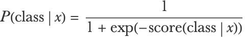
The cost to minimize is then given by the negative log-likelihood:
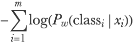
xi and classi are the feature vector and class of training example i and m is the number of training examples. An L2 regularization term is generally added (it could be L1 as well), and the overall loss is as follows:
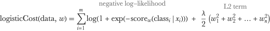
In the linear SVM case, there are no probabilities and we compute the cost function directly from the scores using the so-called hinge loss:
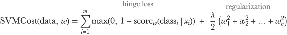
Both cost functions have a term that pushes the model to fit the training data and a regularization term controlled by the hyperparameter λ that pushes the model to have small weights in order to avoid overfitting (note that, by convention, the so-called soft margin parameter ![]() is often used instead of λ, but they are equivalent). Let’s visualize the loss of an example as function of its score for both methods:
is often used instead of λ, but they are equivalent). Let’s visualize the loss of an example as function of its score for both methods:
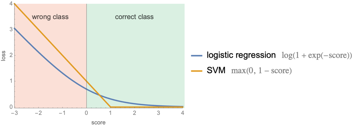
As expected, losses are high for examples with negative scores (misclassifications) and small for examples with positive scores (correct classifications). The SVM loss is particularly simple: it is exactly zero if the score is larger than 1 and linearly increases for smaller scores. It is interesting that examples with scores between 0 and 1 still have a positive loss although they are correctly classified. As a consequence, the linear SVM tries to push such examples further from the boundary by adapting the weight vector w. In a sense, SVM is trying to find a boundary that separates the data with some margin, which is why SVM is also called a large margin classifier. The loss of logistic regression behaves similarly but in a smoother fashion.
Overall, these two losses are quite similar, which means that linear SVM and binary logistic regression are pretty much the same method. Depending on the implementation and size of the data though, linear SVM might be faster to train, which can be useful. The drawback is that linear SVM does not natively provide probabilities, so we have to calibrate the resulting model (see the Classification Measures section in Chapter 3, Classification).
Linear SVM does not provide many benefits over logistic regression. The area where SVM shines, though, is that it can be efficiently modified into a powerful nonparametric method called kernel SVM. Let’s look at this method.
In this context, a kernel, or kernel function, is a kind of similarity measure, which means that it is a function that computes how similar two examples are. For example, if x and x′ are two examples and k is a kernel, k (x,x′) would return a number. A classic example of a kernel is the radial basis function kernel (RBF kernel), a.k.a. squared exponential kernel or Gaussian kernel:
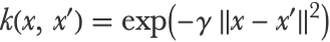
Here x and x′ are numeric feature vectors, x-x′ is then the Euclidean distance between x and x′, and γ is a scaling parameter. This particular kernel can be expressed as function of δ xx-x′. Let’s visualize it for a two-dimensional feature space and for γ=1:
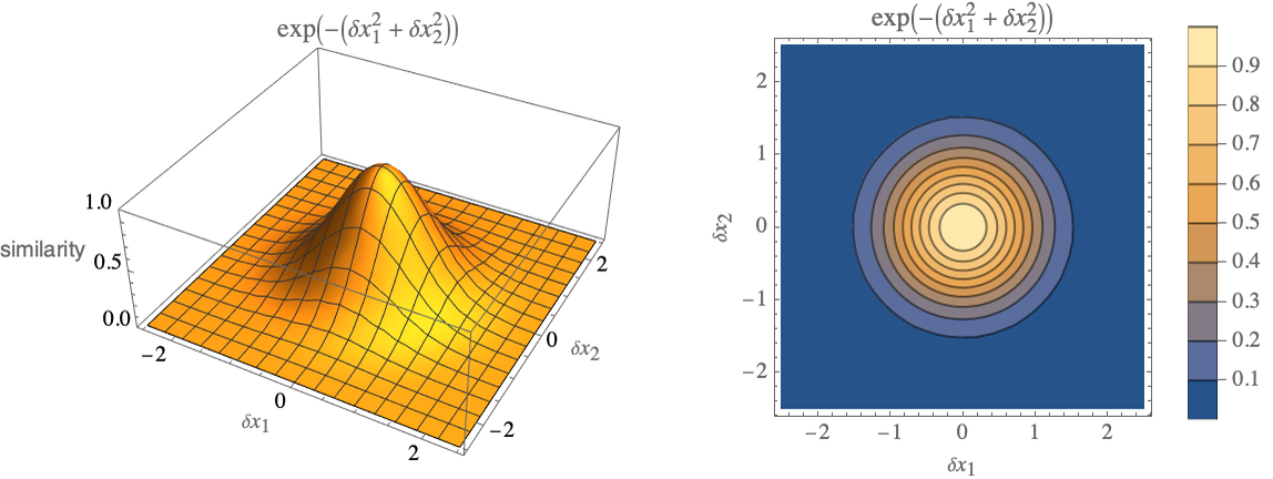
We can see that the maximum is 1 when x=x′ and values quickly fall to zero when the distance between x and x′ gets larger than 1 (and generally, larger than ![]() ), so this is a sort of neighbor detector.
), so this is a sort of neighbor detector.
Kernel SVM uses such kernel functions to extract features. If {x1,x2,…,xm} is the list of all training inputs, a given input example x is transformed into:

This is a vector of features corresponding to the similarity of x with all the training examples. In the case of an RBF kernel in low dimension, this vector would show values around 1 for neighbors and around 0 for others. This feature extractor is used at the beginning of the learning process in order to transform all training examples. The training set thus becomes an mm matrix (the same number of features as the number of examples) called a Gram matrix. This new training set is then given to a linear SVM in order to learn a classifier from it. The resulting model is a linear combination of these kernel features:

Let’s train an SVM with an RBF kernel on the irises dataset limited to classes setosa and versicolor and visualize the scores for the versicolor class:
We can see that each training example locally contributes to the score with its kernel function, with a positive contribution for versicolor examples, and with a negative contribution for setosa examples. The overall model behaves similarly to a nearest neighbors classifier. The size of the kernel is pretty small here because we intentionally set γ=100. With γ=1, the overall score and decision boundary are smoother:
γ can be seen as a regularization parameter that needs to be tuned, in the same way as λ (or C).
In the model with γ=1, many of the learned weights are exact zeros, which means that the corresponding training examples are not used to define the model. The remaining training examples that are used in the final model are called support vectors because they are the “vectors” (i.e. examples) that “support” (i.e. define) the model. These sorts of representative examples are generally, but not necessarily, close to the boundary. The fact that only a fraction of the examples is necessary to perform classification is a major advantage over nearest neighbors since it leads to smaller, faster, and usually better models. SVM with kernels can be seen as a hybrid between an instance-based model and a parametric model (although technically, it is nonparametric).
The resulting model is linear in the kernel feature space but nonlinear in the original space. The features computed using a kernel are generally better than the original features (especially when the original number of features is small), which is why this kernel SVM method works better than the linear SVM. In a sense, this method is using the good assumptions that nearest neighbors does but is improving on nearest neighbors by learning the influence of each training example. Other methods, such as logistic regression, can also be used on such kernel features to improve their performance, but the learning procedure is typically much slower than for SVM and might not result in a sparse model (no support vectors).
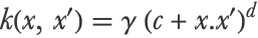
Other kernels than the RBF kernel can be used, such as the polynomial kernel (γ, c, and d are hyperparameters):
Or simply the linear kernel (which gives the linear SVM method):
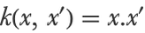
Each of these kernels comes with its own set of hyperparameters, which needs to be tuned in some way.
Custom kernels can also be defined, which can be useful for taking advantage of a specific dataset. However, it is not as straightforward as defining an arbitrary similarity for the nearest neighbors method. Indeed, SVM kernels must satisfy some mathematical properties (being symmetric and positive definite). One way to create such custom kernels is to combine existing valid kernels (such as adding them or multiplying them). In practice, SVM is mostly used with classic kernels, and most of the time, it is an RBF kernel.
We only defined the SVM method for a binary classification problem. Any binary classification method can be extended to work on multiple classes, such as by training many binary models to distinguish a given class from the rest of the classes. These multiclass extensions are generally directly implemented in the libraries. The SVM method can also be extended to work on regression problems, although it tends to be mostly used on classification problems.
The models generated by the kernel SVM method are reasonably small and fast to run because only support vectors are used. On the other hand, the training time can be prohibitive when the number of training examples is important since the method needs to compute the similarities between every pair of training examples.
SVM is an interesting mix of a parametric and a nonparametric method. While not as dominant as it used to be, it can still be a useful method for solving some machine learning problems.
Gaussian Process
Let’s now look at the Gaussian process method, which is a nonparametric Bayesian method that is mostly used for the regression task. This method works well on small datasets and has the advantage of delivering excellent prediction uncertainties. The Gaussian process is not as general purpose as the other methods we have seen so far. It is generally used for some specific applications, such as modeling robot dynamics, forecasting time series, or performing Bayesian optimization.
Using the Gaussian Process
The Gaussian process method uses Bayesian inference to make predictions, which means that a prior over possible model is updated to deduce our belief about the model (see Chapter 12, Bayesian Inference). The name of this method comes from the prior used, a Gaussian process, which is a kind of distribution over functions (see the next section). Before seeing how this method works in more detail, let’s see what kind of model the Gaussian process method produces. Let’s train a Gaussian process on a simple regression task:
As usual, we can use this model to make predictions or obtain a predictive distribution:
The predictive distribution is a Gaussian here, nothing new so far. Let’s now visualize the predictions for a range of values, along with their 68% confidence interval (one standard deviation from the mean):
We can see that the predictions form a smooth interpolation between the training examples, and the training examples are predicted perfectly. This perfect training prediction is not always the case when using this method, but it is a hint that the model is instance based: a prediction is made according to how similar an input is to the training examples. In a sense, the Gaussian process method is an extension of the nearest neighbors method.
Another thing to notice on this plot is that, unlike most other methods, the confidence interval does not have a constant size. The uncertainty is small near the training examples and large in between. Intuitively, this behavior makes sense because we have more knowledge about the true function near the training examples than far from them. This proper modeling of this kind of uncertainty, the one caused by a lack of training data (see the Why Predictions Are Not Perfect section of Chapter 5, How It Works) is an attractive aspect of this method, and it is crucial for some applications.
We said that the Gaussian process method is instance based. More precisely, it is a kernel method, like SVM. This means that the predictions are made using a particular kind of similarity function called a kernel, which in this context is called a covariance function. In our example, the model uses the classic squared exponential covariance (which is another name for the RBF kernel):
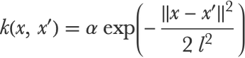
Here, x and x′ are two examples, and α and l are hyperparameters that are automatically determined through a specific optimization process (in principle, it could also be done through cross-validation). This hyperparameter estimation is considered to be the training phase of the Gaussian process method.
Once the model is trained, predictions are made by comparing the example to predict with all of the training examples using the covariance function and using these similarities to combine label values. As a consequence, both training and inference can be very slow when the number of training examples is large. Also, as for other instance-based models, the entire training set has to be stored.
It is possible to choose another type of kernel/covariance in order to obtain better results. Usually, one chooses amongst a set of classic covariances. For example, we could use a linear covariance such as:
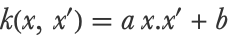
On our previous problem, this covariance gives a different (and probably better) model:
It is also possible to define custom covariance functions, but they have to satisfy some mathematical properties (i.e. to be symmetric and positive-definite, like for SVM kernels). In practice, a simple way to create a custom covariance is to combine classic covariances by adding and multiplying them. For example, we can combine a periodic and a linear covariance to fit data that has a periodic and linear component:
The resulting model is better than with the default covariance (squared exponential) and has good extrapolation abilities, which is attractive for modeling time series. The possibility of creating such structured covariances broadens the capability of the Gaussian process method and allows us to bring knowledge that we might have about a particular problem.
The Gaussian process is not limited to unidimensional data. Here are its predictions on the housing price problem:
This method can also be extended to classification, dimensionality reduction, and even distribution learning. In practice, regression tends to be the most common task for this method though.
Overall, the Gaussian process method allows for the obtaining of good models on small and low-dimensional datasets. Thanks to its proper handling of “lack-of-examples uncertainty,” it is the method of choice for some specific applications, such as Bayesian optimization. Finally, the ability to customize covariance functions allows for the injection of knowledge into the problem and the obtaining of better results. The main drawback of this method is that it is slow to train and slow to make predictions when the number of training examples is too important.
How the Gaussian Process Works
Let’s now dive into how the Gaussian process method works in more detail. Understanding this section is not really necessary for practical purposes (seeing the Gaussian process method as a smart nearest neighbors for which we can define similarity functions is generally good enough). However, the inner details of how this method works are quite interesting, and it can be useful for advanced users or for academic purposes.
The Gaussian process method is based on Gaussian processes, which are a type of random function generator. Random functions (a.k.a. stochastic process, random process, or random field) can be generated in many ways, for example, using random walks:
This random walk effectively defines a particular distribution over functions, which can, for example, be used to model stock prices. Gaussian processes do not generate functions with a random walk but with a multivariate Gaussian distribution (a.k.a. normal distribution), which is where their name comes from. To understand this, let’s define a Gaussian distribution over five variables y1, y2,...,y5. We first need to define the mean value of the distribution, which we choose to be 0 for every value:
Then we need to define its covariance matrix, which defines how variable pairs are correlated:
In this case, correlations are high and positive around the diagonal and go to zero away from it:
This means that y1 is mostly correlated with y2, y2 with y3, etc. Note that a covariance matrix is not exactly a correlation matrix since the diagonal elements do not have to be equal to 1. From this mean and covariance, we can define the full Gaussian distribution:
Let’s now interpret each of these variables as the output of a function f for some discrete inputs: f(1)=y1,f(2)=y2,...,f(5)=y5. The multivariate distribution is now a distribution over discrete functions. Let’s generate random samples from this distribution:
We can visualize the corresponding discrete functions:
We can see that these functions are spatially correlated (they are not wiggling too much) because we chose this particular covariance matrix.
We can extend this distribution to more variables to have smaller gaps between possible inputs. In the infinite limit, the functions are continuous and the distribution becomes, by definition, a Gaussian process. In a sense, a Gaussian process is an infinite-dimensional multivariate Gaussian distribution. Since there are infinitely many variables, the covariance matrix becomes a covariance function, which can also be seen as a kernel (a similarity function). The covariance function defines the correlation between f(x) and f(x′) for any value of x and x′. The most common covariance is the squared exponential covariance that we introduced earlier:

This covariance positively correlates values that are spatially close, and the parameter l corresponds to the spatial correlation length of the functions generated. Let’s define an example of such a covariance:
Let’s now define the x values for which we will compute and display random functions:
We can now compute the covariance matrix for these x values (we add a bit of white noise for numeric stability):
We can use this covariance matrix to sample from the corresponding distribution (again with a zero mean) and to visualize the resulting functions:
As expected, the functions generated are locally correlated (with a typical distance of l≃0.7 here), and they are smooth because of this particular covariance function. Using an exponential covariance, for example, would result in something rugged. This can also be extended to higher dimensions. Here is a sample of a two-dimensional Gaussian process (a.k.a. Gaussian random field):
Custom covariance functions can be used as long as they are symmetric and positive-definite, a mathematical property that ensures that the Gaussian distribution does not have impossible constraints to satisfy such as “y1 and y2 are perfectly correlated, y2 and y3 are as well, but y1 and y3 are not correlated at all.”
Gaussian processes can be used to solve regression tasks. The idea is to use this distribution over functions as a prior belief about the correct function and then use Bayesian inference to update this belief according to the training data (see Chapter 12, Bayesian Inference). Simply put, learning is done by conditioning the Gaussian process on the training data. The key element that makes this possible is that conditioning a Gaussian process gives another Gaussian process (in the same way as conditioning a Gaussian distribution gives another Gaussian distribution). Everything can be computed exactly using linear algebra formulas while most non-Gaussian priors would result in needing to do approximations. Let’s use the one-dimensional prior that we defined earlier and imagine that we only have one training example in our dataset, {x,y}={2,0.5}:
The new covariance matrix for the x values can be directly computed from the previous covariance using the conditioning formula of Gaussian distributions:
We can see that the correlation between f(x=2) (index 40 in the matrix) and other values is zero (the white lines) because this value is already known. Also, the sign of the correlations changes after the known value. Let’s now compute the new means of the x values:
These mean values are the predictions of the Gaussian process. Note that these predictions can be seen as an average of the known values (ytrain) weighted by their similarity in input space with the example to predict (cov〚xtrain,xtrain〛), which is why we described the Gaussian process method as an advanced nearest neighbors.
Let’s visualize these predictions along with samples from this updated process:
As expected, every sample crosses the known value because conditioning is equivalent to selecting the functions that agree with the data. We can see that the mean (predictions) has changed; it now crosses the known value as well.
Let’s add a few extra training examples and visualize the updated covariance matrix:
Again the covariance is zero for known values. Let’s now visualize the updated process:
The samples and the mean cross all training examples, and the samples deviate from the mean between the training examples, which reflects the uncertainty about the predictions. This “envelope” of samples defines the confidence interval that we saw earlier, and it is caused by a lack of training examples. We should note that there are other kinds of uncertainties, such as noisy output values (see the Why Predictions Are Not Perfect section of Chapter 5, How It Works). To account for this possible label noise, a white noise covariance is generally added to the covariance function and ignored when computing the mean (predictions). As a consequence, the predictions do not have to perfectly fit the training data anymore. It is also possible to model this label noise using a more complex covariance instead of a white noise covariance.
We have seen how to make predictions using a Gaussian process. However, the prediction quality depends a lot on the choice of the covariance function and its hyperparameters (l and α in the case of the squared exponential covariance). In principle, we could find a good covariance by using a validation set or through a cross-validation procedure. This procedure is slow and data intensive though, and for Gaussian processes, there is a much better solution. Because it is a Bayesian method, we can directly compute—without using a validation set—which model is better. To understand this, let’s imagine that we only want to pick the best covariance out of two possibilities: cov1 and cov2. We could define a prior for this binary choice, for example, P0(cov1)0.5 and P0(cov2)0.5, and then compute the posterior probabilities for each possibility using Bayes’s rule:

We could then pick the covariance that has the highest posterior probability. In general, the prior P0(covi) is not the most important factor, so we can forget it and just pick the covariance covi for which P(ytraincovi,xtrain) is the highest. P(ytraincovi,xtrain) is referred to as the marginal likelihood because, technically, it is the expected likelihood of the model over the prior defined by the Gaussian process. However, we do not need to compute an expectation to obtain it. It is directly given by the probability for the Gaussian process prior to generate a function crossing the training data exactly. In the case of our three training examples, this is:
It is quite intuitive when you think about it: the best covariance is the one most likely to produce a function that fits the data perfectly. We can thus find the best hyperparameters (or the best covariance type, or even the best combination of classic covariances) by maximizing this marginal likelihood, which can be done in a variety of ways, including through a gradient descent optimization. This optimization procedure is referred to as the training of the Gaussian process.
As we saw, a Gaussian process is a type of distribution over functions that is used as a prior for regression tasks. Gaussian processes can also be used for classification and even for some unsupervised learning applications such as density estimation or dimensionality reduction. A more surprising aspect of a Gaussian process is that it can represent infinite-width neural networks. Indeed, in their infinite-width limit, most neural networks become a Gaussian process whose covariance depends on the structure of the network (and for deep neural networks, one has to stack several Gaussian processes on top of each other). Such models are currently mainly used for research purposes and not so much for practical purposes. Nevertheless, this shows the potential of this method.
Markov Model
Most of the methods we have seen so far are meant to be used on examples that have a fixed number of variables (numerical or categorical). The Markov model method is a classic classification method that is meant to be used on sequences, which are a variable-length ensemble of elements whose order of appearance matters, such as time series, audio recordings, text, or DNA strings. In most cases, the Markov model method is used to classify texts, and it is often called the n-gram method in this context. While modern text applications mostly use neural networks, the n-gram method is still popular for its training speed, simplicity, and ability to obtain decent results when the training data is small and when transfer learning is a not a possibility.
n-Gram Models for Classification
In a nutshell, the Markov model method is based on learning a sequence distribution for each class (see Chapter 8, Distribution Learning) and then using these distributions to classify new sequences. Given a new sequence, the classification is essentially made by picking the class that has the highest probability of generating the sequence. Importantly, the probability distributions are learned using a Markov model, hence the name of the method.
To understand this, let’s use the example of identifying if a text is written in English or in French. As a first step, we are going to learn a distribution for the English language, which is called a language model. For example, let’s consider the following text:
This sentence is a string of 38 characters:
We want to know the probability of this exact sentence being written assuming it is written in English. This is the probability that an English sentence contains all these characters in this exact order:

A way to understand this is to imagine that we have access to an infinite collection of English text documents (similar to existing ones). The sentence probability would then be the probability of obtaining this exact sentence when extracting 38 consecutive characters from this corpus. In principle, one could compute it by counting how many times the sentence appears in a corpus. The problem is that the dataset would need to be extremely large since this sentence rarely appears (in fact, it is likely that it had never been written before), so we must add assumptions, or, in other words, we need to use a model.
A first assumption that we can make to model these sequences is to suppose that characters are generated independently from each other. This is commonly referred to as a bag-of-words assumption, even though it should be a “bag-of-characters” here. The probability is now a product of character probabilities:

This model is much easier to estimate because we only have to measure the frequency of each character in the training set since we don’t care about their correlations. Since we only count single characters, this model is also called a unigram model because an n-gram is a sequence of n characters. Let’s estimate these frequencies on a corpus constituted of Wikipedia pages (to simplify the problem, we transform everything into lowercase and remove diacritics):
We can now extract the characters, count them, and normalize their counts to obtain probabilities:
Let’s visualize these frequencies in a word cloud:
We can see that the letter “e” is present 9.4% of the time, the letter “t” 7.2% of the time, etc. This set of frequencies constitutes a simple yet valid language model. We can, for example, generate a random snippet of English according to this model:
As you can see, the English is not great, to say the least. This is because we ignore correlations between subsequent characters. The distribution of individual characters is correct, however, and for some applications, that might be enough. For example, let’s use this language model to estimate the probability of our fish-dolphin sentence:
This is a small value, but it is normal since there are many possible strings of this length. Now let’s perform the exact same procedure but using a French corpus instead of an English one:
This probability is about 10000 times smaller than what we had before. This means that the English language is much more likely to generate the target sentence than the French one. English should probably be the prediction of the model. Let’s confirm this intuition by computing the probability of the sentence being in a given language P(languagesentence) since we have only computed P(sentencelanguage) so far. To achieve this, we use the Bayesian theorem (see Chapter 12, Bayesian Inference) that states that:

So if we assume the same prior for both classes (P0(English)P0(French)0.5), we can compute P(languagesentence) by simply normalizing P(sentencelanguage):
This means that according to our model, there is a 99.99% chance that the sentence “the red fish was bigger than a dolphin” is English and not French.
The model that we created is rather naive. We can improve upon it by considering the previous character when generating the next character. Mathematically, the sentence probability is now a product of conditional probabilities:

Each of these conditional probabilities can be computed by dividing a bigram probability by a unigram probability:
We, therefore, need to estimate bigram frequencies, which is why this model is called a bigram model. Let’s estimate these frequencies on the English corpus:
As before, let’s visualize them in a word cloud:
We can see that the most frequent pair is an “e” followed by a space. Let’s generate text with this new language model. We can do this by iteratively adding characters to a string, each character being sampled according to P(characterprevious character):
The English is not great still, but at least it is more pronounceable. Let’s use this model to assess the probability of our sentence:
This probability is now much higher than with the unigram model, and this is typical. A better language model tends to give higher probabilities for “correct” texts and lower ones for incorrect texts, such as texts from a different language. Let’s now compute the same probability using the French corpus:
The ratio between both probabilities is now about 108; the sentence is better classified than before. If we were to test this bigram classifier on a test set, we would probably obtain better results than with the unigram classifier.
We could continue to increase the complexity of the model further by using trigrams, 4-grams, etc., but as the complexity increases, we also have to add proper regularization in order to avoid overfitting the data. Many regularization techniques (called smoothing in this context) are possible and some work better than others. The simplest one is the Laplace smoothing, which just involves adding a constant value to the counts of all possible n-grams in order to smooth their frequency estimation. The most effective, at least for modeling text, is called Kneser–Ney smoothing, and it involves combining information from models of different complexity.
We used character tokens here. We could have used other kinds of tokens, such as words, in order to obtain better results (see Chapter 9, Data Preprocessing). Using characters works well for identifying languages, but words are usually better for identifying things like topics, for example.
From Autoregression to Markov Models
Okay, now that we have seen how to train and use n-gram models for text classification, let’s take a step back and define more formally what a Markov model is and its relation to a more general class of models called autoregressive models.
As we said, a Markov model is a distribution over sequences. Let’s call x1,x2,...,xp the p elements of a sequence. The probability for this specific sequence can be written as follows:
This probability can always be decomposed in the following way:

There is no approximation here; it is just a way to rewrite the distribution as a product of conditional distribution of the form P(xixi-1,xi-2,...), which is the distribution of the next element given previous ones. Most sequence models (such as the Markov model, but also recurrent neural networks) attempt to model this distribution P(xixi-1,xi-2,...), which means that they are trying to predict the next element given the past elements of the sequence. These sequence models are called autoregressive because they use their own previous predictions to predict what happens next.
In order to predict the next element of a sequence, say xi, it is intuitive that the previous element xi-1 is probably more important than xi-2, which is more important than xi-3, and so on. The Markov model of order 1 takes advantage of this fact and makes the radical choice of ignoring all elements but xi-1. In a sense, this model has no memory. The probability distribution is now:

Often, this distribution is represented by the following diagram, which is a probabilistic graphical model:
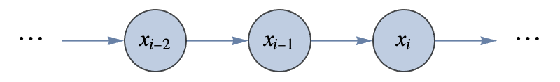
Here, each arrow represents which element is conditioned by which other element. Really, this is just another way to write P(x1)P(x2x1)P(x3x2)...P(xpxp-1). Since each element only depends on the previous one, the generation of a sequence is exactly a Markov chain, a random walk without memory except its current state (see Chapter 12, Bayesian Inference), and that is where the name “Markov model” comes from.
As we have seen, this model can be extended by incorporating additional past elements to predict the future. For example, in a Markov model of order 2, each element is conditioned on its previous two elements:
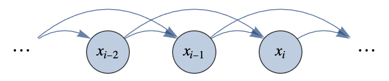
Now the model has a (slightly) larger memory and can make better predictions about what comes next. The sequence generation on the elements is not a Markov chain anymore, but it can still become a Markov chain if we consider pairs of elements ({x1,x2}{x2,x3}{x3,x4}...), which is why it is still called a Markov model.
The Markov model is a fundamental model of machine learning and signal processing in general. A related model is called a hidden Markov model, which allows for the inference of the values of a sequential process when we only observe a noisy version of these values:
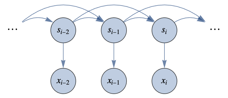
Here, the s values follow a Markov model and produce the x values, which are observed. The s values (also known as the hidden state of the model) are usually not observed, and the goal is to deduce them from the x values. Such a model is not often used in machine learning, but it is heavily used in other areas, such as signal processing.
Markov models are fast and simple. Their downside comes from their small memory of what happened in the past of the sequence. We can increase the order of the model, but it requires more data to obtain good probability estimation. In practice, it is rare to create a Markov model with an order higher than 5 or 6. A solution to this is to use recurrent neural networks or transformer networks (see Chapter 11, Deep Learning Methods), which can also learn to generate sequences in an autoregressive way but can remember things further in the past.
| ■ | Classic machine learning methods are heavily used to tackle structured data tasks. |
| ■ | Classic machine learning methods are usually fast and easy to use. |
| ■ | Neural networks are better than classic machine learning methods for unstructured data tasks. |
| Linear regression | |
| ■ | Linear regression is a parametric regression method. |
| ■ | Linear regression predicts using a linear combination of features. |
| ■ | Linear regression is used for its speed and simplicity. |
| ■ | Linear regression requires good feature engineering. |
| Logistic regression | |
| ■ | Logistic regression is a parametric classification method. |
| ■ | Logistic regression classifies using linear combinations of features. |
| ■ | Logistic regression is used for its speed and simplicity. |
| ■ | Logistic regression requires good feature engineering. |
| Nearest neighbors | |
| ■ | Nearest neighbors is a nonparametric method for classification and regression. |
| ■ | Nearest neighbors predicts by finding similar training examples. |
| ■ | Nearest neighbors does not require a training procedure. |
| ■ | Nearest neighbors requires the storing of the entire training set. |
| Decision tree | |
| ■ | Decision tree is a nonparametric method for classification and regression. |
| ■ | Decision tree predicts by asking several true/false questions about the features. |
| ■ | Decision tree is used when interpretability is required. |
| Random forest | |
| ■ | Random forest is a nonparametric method for classification and regression. |
| ■ | Random forest uses an ensemble of decision trees to make predictions. |
| ■ | Each decision tree is trained independently on a variation of the training set (bagging procedure). |
| ■ | Random forest has very few hyperparameters. |
| ■ | Random forest is one of the best classic machine learning methods. |
| Gradient boosted trees | |
| ■ | Gradient boosted trees is a nonparametric method for classification and regression. |
| ■ | Gradient boosted trees uses an ensemble of decision trees to make predictions. |
| ■ | Decision trees are trained sequentially to correct the errors of their predecessors (boosting procedure). |
| ■ | Gradient boosted trees has many hyperparameters. |
| ■ | Gradient boosted trees is considered the best classic machine learning method. |
| Support-vector machine (SVM) | |
| ■ | SVM is a nonparametric method for classification and sometimes regression. |
| ■ | SVM predicts by comparing training examples using a kernel. |
| ■ | A kernel is a kind of similarity function. |
| ■ | SVM learns a weight for each training example. |
| ■ | SVM used to be the dominant classic machine learning method. |
| Gaussian process | |
| ■ | Gaussian process is a nonparametric method for regression and sometimes classification. |
| ■ | Gaussian process predicts by comparing training examples using a covariance function. |
| ■ | A covariance function is like a kernel, which is a kind of similarity function. |
| ■ | Gaussian process is excellent at modeling the uncertainty caused by a lack of training examples. |
| ■ | Gaussian process is used for applications requiring good prediction uncertainties. |
| ■ | Gaussian process is slow to train and slow to make predictions. |
| Markov model | |
| ■ | Markov model is a method for sequence classification, such as text classification. |
| ■ | For text, Markov model computes class probabilities using the n-gram frequencies of the sequence. |
| ■ | Markov model is an autoregressive method with a small memory. |
| ■ | Markov model is used to classify text when data is small and when transfer learning is not possible. |
| linear regression | regression method making predictions using a linear combination of features | |
| weights | alternative name for the parameters of a model, principally used for neural networks | |
| intercept bias | constant term added after a linear transformation | |
| L1 regularization L1 penalty | classic regularization strategy for parametric models, penalize large parameters in the cost function, can lead to parameters being exactly zero | |
| L2 regularization L2 penalty | classic regularization strategy for parametric models, penalize large parameters in the cost function | |
| convex function | differentiable real-valued function whose (hyper)surface is above all its tangent (hyper)planes, does not contain local minima besides the global minimum | |
| maximum likelihood estimation | estimation of the optimal parameters of a probabilistic model by maximizing the likelihood of the model on some data |
| logistic regression logit regression softmax regression maximum entropy classifier | classification method predicting class probabilities using a linear combination of features | |
| multinomial logistic regression | logistic regression with more than two classes | |
| softmax function LogSumExp function | function that transforms any score vector into a valid categorical distribution, applies an exponential to the scores and normalizes the result | |
| partition function | normalization part of the softmax function, term originates from statistical physics | |
| logits | scores before application of the softmax function | |
| linear classifier | classifier that separates each class pair by a linear/planar decision boundary |
| nearest neighbors | classification and regression method that makes predictions according to the nearest examples of the training set | |
| Laplace smoothing additive smoothing | smoothing method to estimate categorical distributions, add a count value to all possible categories | |
| nonlinear model | any model that does not simply use a linear combination of features | |
| lazy learning | not computing anything at training time, delaying potential computations at evaluation time |
| decision tree | classification and regression method that makes predictions by asking questions about the value of the features | |
| knowledge distillation | training a model on the predictions of another model, used to reduce model size |
| random forest | classification and regression method that uses an ensemble of regression trees trained using the bagging procedure | |
| ensemble of decision trees decision forest | set of models that are combined to form a better model | |
| bagging (bootstrap aggregating) | using bootstrap samples (resample with replacement) to create an ensemble of models | |
| resampling with replacement | randomly selecting a set of examples from a dataset, examples are sampled independently from each other so there can be duplicates in the resampled set |
| gradient boosted trees | classification and regression method that uses an ensemble of regression trees trained using the boosting procedure | |
| boosting | creating an ensemble of models by sequentially training models to correct the errors of previous models |
| support-vector machine large margin classifier | nonprobabilistic classification method that classifies by comparing training examples using a kernel function | |
| kernel function | similarity measure between data examples | |
| hinge loss | loss function used to train support-vector machines | |
| linear SVM | linear version of the support-vector machine method | |
| kernel SVM | support-vector machine method that uses kernels to create features | |
| support vectors | all training examples that define a given support-vector machine model | |
| radial basis function kernel squared exponential kernel Gaussian kernel | most common kernel, uses a Gaussian distribution to define similarity |
| random functions stochastic process random process random field | distribution over functions | |
| Gaussian process | specific kind of random functions, infinite-dimensional Gaussian distribution | |
| Gaussian process method | Bayesian nonparametric regression method that uses a Gaussian process to define a prior distribution over models | |
| covariance matrix | matrix giving the covariance between all pairs of data examples, can be used to define a multinormal distribution | |
| covariance function | continuous version of the covariance matrix that gives the covariance for any pair of data examples and can be used to define a Gaussian process, same as a kernel function but for a different use | |
| squared exponential covariance | most common covariance function, uses a Gaussian distribution to define similarity | |
| marginal likelihood | expected model likelihood over the prior of the model |
| sequential data | variable-length ensemble of elements whose order of appearance matters, such as time series, audio recordings, text, or DNA strings | |
| language model | distribution over textual data, the model is able to generate text or estimate the probability of a given text | |
| autoregressive model | sequential model that uses its own previous predictions to predict the next elements of the sequence | |
| Markov model | autoregressive model with a fixed-length memory | |
| n-gram | sequence of n categorical tokens | |
| Markov model method | sequence classification method that uses Markov models to learn a sequence distribution for each class, called the n-gram method when applied to categorical sequences | |
| Kneser–Ney smoothing | effective smoothing technique for Markov models | |
| hidden Markov model | model that allows for the inference of the values generated by a Markov model when we only observe a noisy version of these values | |
| probabilistic graphical model | distribution for which a graph expresses the conditional dependence structure between random variables |