Now that we know how to create classifiers and regression models, let’s try to understand what is happening under the hood. Knowing every detail of how machine learning works is not necessary to use machine learning, but it is important to have a general understanding of it. Such understanding allows us to be aware of the strengths and weaknesses of machine learning, to figure out where machine learning can be applied, and to create better machine learning models overall.
Model
At the core of machine learning is the concept of a model, which was already mentioned. Let’s look at this concept in more detail.
In the mathematical sense, a model is a description of a system. Models are used in most scientific and engineering disciplines as tools to analyze, predict, or design things. For example, an engineer might create a model of a building to predict its behavior and improve its structure, an economist might create a model of a city to help urban planning, and a climatologist might create a model of Earth’s climate to predict its evolution.
In the context of machine learning, we are generally interested in making predictions. Such predictive models can, for example, describe how a variable y (such as a quantity or a class) is related to other variables, let’s say x1 and x2:
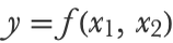
Here the model is represented by the function f. This function only returns a prediction in this case, but it could similarly return probabilities or continuous distributions as we saw in previous chapters. There are many ways to define such a function; it could be done through a mathematical formula such as:
Let’s use this formula to make a prediction:
A model can also be defined by a neural network such as:
This network can compute something from an input:
And a model could even be defined by a classic computer program:
Let’s run this program on a given input:
Using a model is generally easy; the difficult part is creating it. Ideally, we would want to obtain a model that perfectly describes whatever system we are interested in. In practice, that is not possible. Models cannot be perfect, but they can still be useful as long as they are not too far from reality (this is summarized by the famous dictum, “All models are wrong, but some are useful”). Sometimes unrealistic models can even be more useful than realistic ones if they are simpler, faster, or easier to work with.
The traditional modeling approach (i.e. without machine learning) is to use a theory about how the system of interest works (e.g. the principles of mechanics) and to develop a model “by hand.” This is similar to the classic programming approach described in the first chapter. In machine learning, however, the model is created by the computer using data.
How can a computer create, by itself, a good model? There are several machine learning methods that have names like “decision tree,” “linear regression,” or “neural networks,” which are described in more detail in Chapter 10, Classic Supervised Learning Methods, and Chapter 11, Deep Learning Methods. In a nutshell, many of these methods can be seen as a search process: the computer is given a class of possible models and it then “searches” for the best one amongst this class. The key is that computers can quickly measure a model’s performance by testing their predictions against the data. Once you can measure a model’s performance, you can compare models, and it is just one step forward to find a good model. You just need to search for it. One naive way to search is to evaluate the performance of many random models and to select the best one. A less naive version is to iteratively modify an initial model. Developing ways to search more efficiently, which is called optimization, is an active research area.
Another important point is that the computer needs a class of models to start with. Indeed, searching amongst “every possible model” would require an infinite amount of time and data. The computer, therefore, needs to be restricted to a certain class of models (often called a model family), and the choice of this class greatly affects the final performance. Finding “good” classes of models is the main focus of machine learning research. Note that the term “model” is often actually used to refer to a model family, or even to a complete machine learning method, but not necessarily to refer to a specific trained model.
Machine learning methods are generally separated into two groups: parametric methods and nonparametric methods. In the next sections, we will create models from scratch in order to understand what these groups are.
Nonparametric Methods
Nonparametric methods are machine learning methods whose model size varies depending on the size of the training data. They are named in opposition to parametric methods (see the next section), which generate models that have a fixed set of parameters. As we will see, nonparametric methods are amongst the most intuitive machine learning methods.
Models generated by nonparametric methods are called nonparametric models, and most of them can be seen as instance-based models (also known as memory-based models, neighbor-based models, or similarity-based models). Instance-based models make predictions by finding similar examples in the training set. To understand this better, let’s create one of these models from scratch.
First, we load the classic MNIST dataset, which is composed of images of handwritten digits that are labeled by their corresponding digit:
Here are 10 examples:
Let’s extract images and labels from this dataset:
This dataset is composed of 60000 examples and is balanced in terms of class counts:
Our goal is to create a classifier that can recognize handwritten digits. In other terms, we want to obtain a function f such that ![]() returns “2,”
returns “2,” ![]() returns “6,” and so on. To make the problem simpler, we will focus on only the image
returns “6,” and so on. To make the problem simpler, we will focus on only the image ![]() for now.
for now.
Let’s first understand what images are. A digital image is a collection of pixels. In this dataset, each image has 28 pixels in each direction, so there are 784 pixels in total:
Each pixel color is defined by numbers. In our case, each color is a shade of gray, so it is just one number. For example, the number 0 corresponds to black, 1 to white, and every number in between corresponds to a shade of gray:
Let’s extract pixel values from our unlabeled image:
As expected, these values form a matrix of size 2828:
Note that most of these values are exactly 1 because the background of the image is white. To simplify things, let’s transform this matrix into a vector:
The image is now a list of values called a feature vector because each value would be considered a feature by machine learning methods. Most classic machine learning methods require the data to be transformed into such vectors.
Okay, so we now have a vector of 784 values, and we want to guess the label. One simple assumption we can make is that similar images tend to have similar labels. We can measure if two images are similar by computing the Euclidean distance between their feature vectors:
This is called a pixel-wise distance. Let’s use this distance to find the training images most similar to our unlabeled image ![]() . We first need to transform training images into vectors:
. We first need to transform training images into vectors:
We can now compute distances between our image vector and all training vectors:
From these distances, we can identify the nearest training image along with its corresponding label:
As you can see, the nearest training image to ![]() is
is ![]() and has the label “4,” which is encouraging! A naive strategy would be to always return the label of the nearest training image. Here is a program that implements this predictive model:
and has the label “4,” which is encouraging! A naive strategy would be to always return the label of the nearest training image. Here is a program that implements this predictive model:
Let’s use this model on images that were not in the training set:
As you can see, the model works surprisingly well. This method is called nearest neighbors and, as simple as it is, it can already solve many machine learning problems. There are many things that we could do to improve upon it. For example, we could take several neighbors instead of only one and choose the most common class within these neighbors. Here is a sketch of what this process would look like in a two-dimensional space (two numeric features):
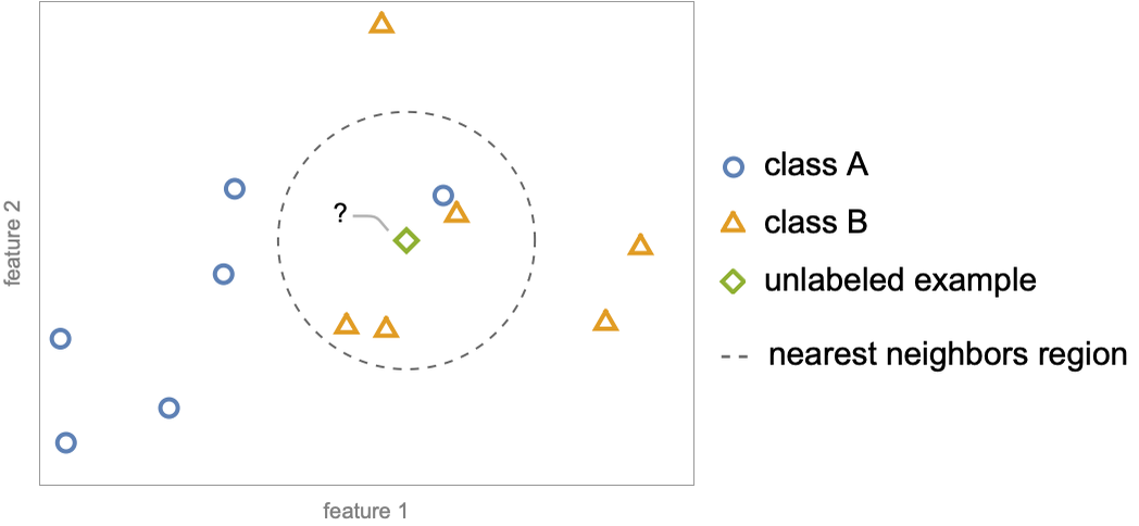
Amongst the four nearest neighbors of the unlabeled example ![]() , one belongs to class A (
, one belongs to class A (![]() ) and three belong to class B (
) and three belong to class B (![]() ), so the prediction is class B. This version is called k-nearest neighbors, also known as k-NN (k refers to the number of neighbors taken). k-nearest neighbors can also be applied to a regression problem; the prediction would simply be the average of the labels of the nearest neighbors. Here is an example (with k=1) applied to a simple regression problem:
), so the prediction is class B. This version is called k-nearest neighbors, also known as k-NN (k refers to the number of neighbors taken). k-nearest neighbors can also be applied to a regression problem; the prediction would simply be the average of the labels of the nearest neighbors. Here is an example (with k=1) applied to a simple regression problem:
The training data is the points in blue and the prediction curve is shown in red. As you can see, predictions are just a copy of the output values of the nearest neighbor because k=1.
k-nearest neighbors is the simplest kind of instance-based models. There are several others. Here is an example of another instance-based model called the Gaussian process (see Chapter 10, Classic Supervised Learning Methods) applied to the same regression problem:
As we can see, the model performs a smooth interpolation between training examples (and the uncertainty about the prediction grows as one moves away from the training examples). The math behind Gaussian processes is more complex than for nearest neighbors, but in essence, they are similar models. Instance-based models compare new examples to their most similar training examples (the “instances” seen during the training) and they perform some kind of average to obtain a result. These models can be seen as interpolators that fill in the blanks between training examples.
Several other classic methods can (roughly) be seen as instance-based methods, such as support-vector machines, decision trees, or random forests. We detail these methods further in Chapter 10. These methods are heavily used to solve machine learning problems, especially when structured data is involved (such as numeric and nominal variables stored in a spreadsheet or a database). However, these methods tend not to perform so well on images, text, or audio. For such problems, neural networks are typically better. Another drawback of instance-based methods is that they need to store at least a fraction of all training examples, which can be prohibitive in terms of memory and speed.
Nevertheless, instance-based models are always a good way to think about how machine learning works; they are good mental models. As it happens, even neural networks have similarities with instance-based models, for example, modern neural networks trained on image classification tasks tend to obtain perfect results on every training example. In a sense, they memorize training examples and perform some kind of interpolation between these examples (yet they can learn a much better way to interpolate than methods like nearest neighbors).
Parametric Methods
Parametric methods are all machine learning methods that generate models defined by a fixed set of parameters. In machine learning, “parameters” refers to the values that uniquely define a model. Classic parametric methods include linear regression, logistic regression, and neural networks. To understand this better, let’s create some simple parametric models from scratch.
Regression Example
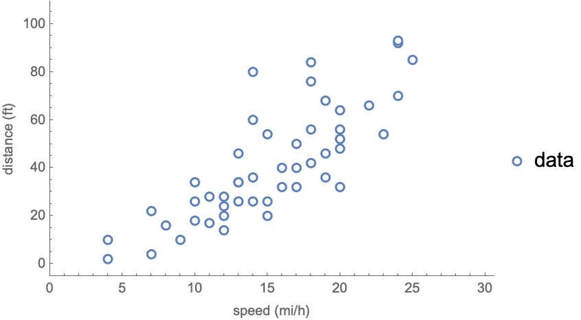
We will use the same Car Stopping Distances dataset we used in Chapter 4, which consists of 50 examples of car stopping distances as function of their speeds:
Let’s visualize this data in a scatter plot:
Our goal is again to predict the stopping distance for a given speed.
In this dataset, the input and output variables are quantities (speed in miles per hour and distance in feet). Let’s extract their numeric values and separate these variables:
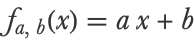
Let’s now define a class of models that will be used to predict the distance given a speed:

This model predicts the distance by multiplying the speed (x) by a constant (a) and adding another constant (b). Programmatically, this model is:
fa, b represents many possible models (that is, a family of models) depending on the values given to a and b, which are the parameters of the model. For example, if a=1 and b=2, the model can predict distances:
Let’s visualize these predictions along with the data:
Of course these predictions are not good; they do not fit the data well. “Fitting” is the usual term for describing the agreement between a model and the data. In this case, the fit is bad because the values for the parameters are not appropriate. We need to figure out better values for the parameters a and b, and we are going to learn these values.
The first thing that we need in order to learn the parameters is to be able to measure the quality of a given model. This measure is called a cost function (it also has other names such as empirical risk and objective function). A cost function is usually a simple formula that compares predictions to data and returns a number. The lower the cost, the better the model. For our problem, we use the mean squared error, which is a classic choice when dealing with numeric predictions (see the Regression Measures section in Chapter 4). In a mathematical form, the mean squared error is as follows:
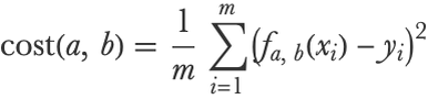
Where xi is the speed of example i (and therefore fa, b(xi) is the predicted distance for example i), yi is the true distance of example i and m is the total number of examples in the dataset. Programmatically, this cost can be written as follows:
x and y are the input and output extracted previously. Note that this cost is an average over the contributions of all examples, so we could also write it like this:
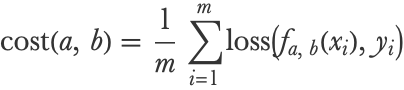
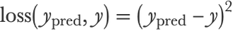
Here we introduced a per-example loss function, which, in this case, would be the squared error loss (a.k.a. quadratic loss):
Often, the terms “cost” and “loss” are used interchangeably, but, in principle, they are different things. Cost is a measure over an entire dataset (and might include regularization terms as we will see later) and loss is a per-example measure.
As we can see, this loss is computing differences between predictions and real values and then squaring these differences in order for them to always be positive. Because of the square function, a small deviation from the data has little effect on the cost while a large deviation leads to a high loss that increases the cost by a lot:
A perfect cost would have a value of 0 here. For a=1 and b=2 the cost is:
To obtain better predictions, we need to find parameters for which the cost is lower. Let’s visualize the value of the cost as function of a and b:
We can see high-valued regions in blue and low-valued regions in red, in which lies the minimum. The task of finding the location of the minimum is called optimization. There are several optimization methods that we could use. The simplest one is to try random values for the parameters. A better one is to iteratively refine the parameters in directions that are decreasing the cost, such as using gradient descent, which is explained in Chapter 11, Deep Learning Methods. For now, let’s just use the automatic optimizer FindArgMin on the cost function:
The learned values are aopt≃3.93 and bopt≃-17.58, which indeed give a lower cost:
The predictions with these parameters are visibly better:
The model now fits the data. We can use this learned model to predict a sensible stopping distance for a car traveling at 23 miles per hour:
And that’s it. We trained and used a parametric model from scratch.
This particular method is called linear regression, and it is the simplest parametric method (see Chapter 10, Classic Supervised Learning Methods). On the opposite end of the spectrum is neural networks, which are also parametric and quite a bit more complex. The learning principle of neural networks is the same though: optimizing parameters to minimize a cost function.
Classification Example
Parametric methods are not limited to regression; they can be used for just about every machine learning task. Let’s train a simple parametric model for classification. We will use the car vs. truck dataset seen in Chapter 3, Classification:
Instead of directly predicting a class, let’s predict class probabilities, which is the usual thing to do. We use the following class of models Pa, b defined by:

This can be written as:
This class of models again has two parameters. Let’s try it with a=1 and b=2 on a given input:
This means that the model gives a 90.9% probability of the class being a car and a 9.1% probability of the class being a truck. Note that these probabilities are between 0 and 1 and that they sum to 1. This is always the case for such models by design. These are logistic regression models (described in more detail in Chapter 10, Classic Supervised Learning Methods), named after the logistic function they use:
The usual cost function for probabilistic classification is the negative log-likelihood, a.k.a. mean cross-entropy (see Chapter 3, Classification). This cost uses the cross-entropy loss (a.k.a. log loss), which means it computes the mean log-probability of the correct classes:
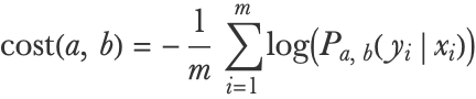
This can be programmatically written as:
This cost pushes the model to assign high probabilities to the correct class and low probabilities to the incorrect class(es), which seems like a sensible thing to do. Let’s find the optimal parameters:
We can now predict the probabilities for new examples:
Let’s visualize the predicted probabilities along with the training data:
As we can see, the two classes have been correctly separated. The model learned to make sensible predictions from the data.
Maximizing the likelihood of probabilistic classifiers is the dominant procedure to train parametric classifiers. This is, for example, how neural network classifiers learn.
Model Generalization
In the previous section, we focused on creating models that fit their training data. However—and this is a crucial point—the goal of machine learning is not to obtain good performance on training data but to obtain good performance on unseen data, which refers to data that was not in the training set.
To understand this better, let’s imagine a handwritten digit classifier that works in the following way. During the training phase, it stores every example in the training set into a lookup table such as:
When given an image, the classifier searches in this lookup table to find if there is an exact match. If there is a match, it returns the corresponding class from the table:
If there isn’t a match, the classifier returns a random digit:
The classifier described above obtains perfect results for training examples, but it cannot recognize images that were not in the training set. This model is therefore useless. In order for a model to be useful, we need it to also work on unseen data. In machine learning terms, we say that models must generalize to unseen data. Generalization is a fundamental property that every machine learning model should have, not just predictive models.
Okay, models need to generalize to unseen data, but what is unseen data exactly? Just about all machine learning methods make the assumption that unseen data comes from the same distribution as the training data. This is called the iid assumption, which stands for independently and identically distributed. This does not mean that the unseen data and training data are the same, just that they have been generated in the same way. In the case of the unseen example ![]() , the iid assumption is probably valid since this example looks like our training examples:
, the iid assumption is probably valid since this example looks like our training examples:
Example ![]() has thus probably been generated in the same way as the training examples. It is said to be in-distribution, or in-domain. The example
has thus probably been generated in the same way as the training examples. It is said to be in-distribution, or in-domain. The example ![]() , however, seems qualitatively different from the training examples. It has been generated differently and is thus said to be out-of-distribution, or out-of-domain. Machine learning methods are assuming that unseen data is in-distribution, which means that their models are not supposed to work for out-of-distribution examples.
, however, seems qualitatively different from the training examples. It has been generated differently and is thus said to be out-of-distribution, or out-of-domain. Machine learning methods are assuming that unseen data is in-distribution, which means that their models are not supposed to work for out-of-distribution examples.
The ability of a model to work well on data coming from the same distribution as the training data is called in-distribution generalization, and it is what machine learning methods focus on. The issue is that the iid assumption is often wrong in practice: the data on which a model is used can qualitatively differ from the training data. Ideally, we would like an out-of-distribution generalization, which means that examples like ![]() should still be correctly classified even when the model is trained on grayscale handwritten digits. In a sense, we would like models that can extrapolate and not just interpolate. A model that can generalize decently on out-of-distribution data is said to be robust while a model that cannot is said to be brittle.
should still be correctly classified even when the model is trained on grayscale handwritten digits. In a sense, we would like models that can extrapolate and not just interpolate. A model that can generalize decently on out-of-distribution data is said to be robust while a model that cannot is said to be brittle.
There is ongoing research to find ways to truly generalize to out-of-distribution data, such as by using causal models or by using several qualitatively different training sets and learning to generalize from one set to another. However, such methods are in their infancy and not much used in practice yet. Practically, the first thing to do to train a robust model is to make sure that the training data is as diverse as possible, such as merging datasets from different origins. Another thing we can do is to preprocess the data in order to ignore irrelevant features or spurious features. Irrelevant features are the features that do not bring information about the label value, and spurious features are the ones that are correlated with the labels in the training data but might not be in the new data due to a data shift (see the section Why Predictions Are Not Perfect in this chapter). A typical example of spurious features in images are textures, which are usually correlated with the label but not always, as opposed to shapes, which are more robust. We could try to remove these irrelevant/spurious features or use a feature extractor that is known to capture semantic features, which means features that capture the “meaning” of the data example well. In any case, it is not possible to obtain a perfectly robust model, so a last resort strategy is to detect when an unseen example is out-of-distribution using an anomaly detector (see Chapter 7, Dimensionality Reduction, and Chapter 8, Distribution Learning) and then return a special output or issue a warning if an anomaly is found.
Okay, even if the iid assumption is satisfied, how can a model learn to generalize? This is not an easy question to answer, and in a sense, this is the main focus of machine learning research. At the fundamental level, it involves using models that, even before being trained, make good assumptions about the data. For example, the nearest neighbors method assumes that similar elements tend to have similar classes, a sort of continuity assumption (and just about all machine learning methods make this assumption). Similarly, neural networks make all kinds of implicit assumptions, such as the fact that data tends to be hierarchical (e.g. a picture is composed of objects, which have different parts, themselves composed of lines, etc.). It is these assumptions that allow models to fit a training set and still perform well on unseen data. These assumptions are referred to by many names, such as learning bias, inductive bias, prior knowledge, or prior hypotheses. In most cases, these assumptions are implicit, but they can also be explicitly defined using distributions (see Chapter 12, Bayesian Inference).
Overfitting and Underfitting
Obtaining good assumptions to generalize well is not straightforward, which is why all of these machine learning methods exist. However, there is one aspect that we can often easily control and which is important to consider: the strength of these assumptions. Indeed, when the number of training examples is small, we need to help the data by making strong assumptions. Otherwise, we would fall into the infamous overfitting regime and obtain models that do not generalize well. On the other hand, if the number of training examples is large, we should not assume too much and let the data speak. Otherwise, we would fall into an underfitting regime and also obtain suboptimal models. Let’s see whether these regimes are using the classic example of polynomial curve fitting.
We first load the Fisher’s Irises dataset and extract two of its numeric variables:
This corresponds to the petal and sepal lengths of 150 specimens of irises. Let’s extract the values from this data and visualize them:
To compare the generalization abilities of models, we need to keep aside data examples that will not be used during the training phase. This can be done by splitting the dataset into a training set and a validation set, sometimes also called a development set. Creating a good validation set (like creating a good test set) is one of the most important tasks of machine learning. As a general rule, the validation set must be as qualitatively different as possible from the training set in order to really test the generalization abilities of models. For example, it is a good idea to use separate data sources to create the training set and the validation set. In our case, we only have one source of data, so we must resort to the poor man’s solution of shuffling the dataset and splitting it in two. Let’s keep 20 examples in the training set and use 130 examples in the validation set (note that the training set is generally larger than the validation set, but here the split is made to obtain good measure uncertainties as opposed to good models):
Here are the resulting datasets:
Let’s now train a linear model as we did before, such as:
Instead of defining a cost function and doing an optimization, we can directly use the function Fit, which minimizes the mean squared error:
This gives the following predictions:
Let’s now compute the cost values (mean squared errors) on the training and validation sets:
We can see that the training cost is lower than the validation cost. This is completely normal because the model has been trained to fit the training set and not the validation set.
Let’s now try to create a better model; that is, let’s try to lower the cost on the validation set. One way to do this is to use a more complex model that should be able to fit more complex variations of the data. We will use a quadratic function:
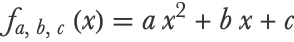
This model has an additional parameter compared to the linear model. Also, note that the quadratic model is equivalent to the linear one if a=0, so it should at least match the fitting abilities of the linear model. This means that the quadratic model defines a broader family of functions; it is said to have a higher capacity and, therefore, should be able to capture more complex data patterns. Let’s train this model and visualize its predictions:
This fit seems a bit nicer. Let’s compare the training costs of both models:
As expected, the training cost of the quadratic model is lower. Let’s now compute the cost on the validation data, which is what really matters:
The validation cost of the quadratic model is lower. This means that up to statistical uncertainties (due to the finite size of the validation set), the quadratic model is truly better than the linear model. We made progress! This also means that the linear model is underfitting the data compared to the quadratic model: its lack of capacity leads to worse performance. Let’s now figure out what happens when we use a model that has a much larger capacity, such as a polynomial of degree 15:
This time things look a bit strange. While the model fits the training examples pretty well (even giving perfect predictions for most of them), the model can give bad predictions between training examples. This is confirmed by computing the cost values:
While the training cost (~0.04) is much smaller than for previous models, the validation cost (~32) is much higher than for previous models. This is a classic example of being in the overfitting regime: we increased the capacity of the model too much and it resulted in worse performance. In a sense, this higher-capacity model has too much freedom for the size of this training set (only 20 examples) and, therefore, starts to fit irrelevant variations of the data (the label noise), which, in this case, harms the generalization abilities of the model. To have a clearer idea of what is going on, let’s now train and visualize the performance for all polynomial degrees up to 10:
We can see that the validation cost follows a U-curve: increasing the capacity is helpful at first, but past a certain point, it becomes harmful. The intuition is that low-capacity models make strong assumptions about the data, and it is, therefore, difficult for them to adapt to the data. Their rigidity is a source of error. On the other hand, high-capacity models make weak assumptions, so it is easy for them to adapt to the data, but the consequence of this flexibility is that they are more prone to fitting the noise of the data. There is, therefore, a tradeoff to make, which in statistics is referred to as the bias-variance tradeoff. Here, bias refers to the learning bias of the model (i.e. its assumptions) and variance refers to the sensitivity of the model to the training data.
In our case, the best model, up to measure uncertainties, is the polynomial of degree 6. This model has the capacity to fit more relevant variations than lower-degree models, but it does not fit much harmful noise yet:
Models with lower degrees (and thus lower capacities) are said to underfit the data, and models with higher degrees (and thus higher capacities) are said to overfit the data.
Controlling the capacity is a key element to obtaining models that generalize well. We should not forget that it is not the full story though. Using qualitatively good assumptions (that is, a good class of models) for the problem at hand is also important to generalizing well.
Regularization
In the previous section, we saw that it is important to control the capacity of machine learning models. Such capacity can be modified by changing the number of parameters, but it can also be controlled in other ways. The process of controlling the capacity of a model is called regularization (and in some contexts, smoothing). The term “regularization” comes from the fact that the usual procedure is to decrease the natural capacity of a model as opposed to increasing it.
Let’s go back to the polynomial fitting example and try to improve the performance of a model in the overfitting regime without reducing the number of parameters. To do so, we modify the cost function by adding a regularization term:
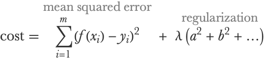
This regularization term is a sum of squares of the parameters (the polynomial coefficients). Since the training procedure minimizes the cost, this regularization term pushes the parameters toward 0. This is called an L2 regularization (or L2 penalty) and is a soft way to reduce the influence of the parameters since they become closer to 0. λ is the value that controls the intensity of the regularization; it is a regularization hyperparameter. Hyperparameters are all the “parameters” of a machine learning method that are not learned during the training procedure and thus need to be set before training.
Okay, so let’s re-train the polynomial of degree 15 with some L2 regularization:
Let’s now compute the validation cost of this new model:
We can see that this cost (0.146) is much smaller that the cost without regularization (31.8), which means that we improved the model a lot by regularizing it. Let’s visualize the new model and compare it with the original one:
Again, things look better for the regularized model. It is much smoother, and it does not fit the noise as much. Using such a regularization strategy is typically better in terms of generalization than reducing the number of parameters, but this is not a fundamental rule.
Here we chose a value of λ=0.1 because it happened to work pretty well after a few tries. Let’s see if we can find a better value for λ. The simplest way to achieve this is to try several values at once that we believe could work, such as:
We can train the corresponding models on the training set and test them on the validation set (as we did to determine the optimal polynomial degree):
Here are the cost values as function of λ:
The training cost increases as expected since we are reducing the capacity of the model. The validation cost, however, follows a U-shape again, and the optimal value is λ=0.1.
L2 regularization is a classic regularization technique of parametric methods. There are several other ways to regularize models. For example, in the k-nearest neighbors method, the number of neighbors k allows for the control of the capacity of the model. Here is an illustration (from the Nearest Neighbors section of Chapter 10, Classic Supervised Learning Methods) of a classifier trained with one neighbor and 20 neighbors:
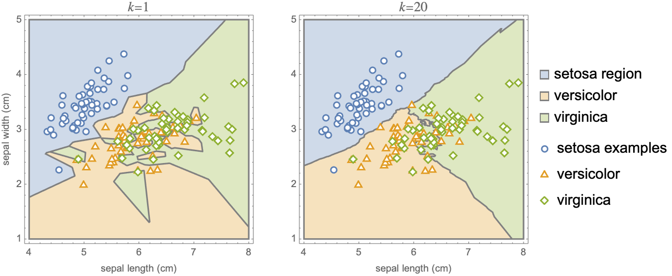
We can see that the classification regions are less fragmented and show fewer variations when the number of neighbors is large.
For neural networks, a simple regularization technique consists of stopping the training before it finishes. To illustrate this, let’s train a network with many parameters on our training data:
The training phase is iterative, so we can visualize how cost values evolved during the training:
We see that the validation cost is decreasing first, and then it starts to increase after about 1600 rounds as the training continues. To obtain the best model, we should, therefore, stop the training at 1600 rounds. This technique is called early stopping, and it is used a lot in practice due to its simplicity (it is not necessarily the best regularization method though). The number of training rounds can be seen as a regularization hyperparameter here.
Regularization is an important component to obtaining good models. Not all regularization techniques are equal though. For example, regularizing a neural network with an L2 penalty, early stopping, or something like dropout (see Chapter 11, Deep Learning Methods) will result in different models. Similarly, bagging decision trees is a much better regularization technique than pruning a single decision tree (see the Random Forest section of Chapter 10, Classic Supervised Learning Methods). One way to interpret regularization is that it adds hypotheses about the model, therefore increasing its learning bias and reducing its variance. Naturally, some hypotheses about the model are just better than others.
Hyperparameter Optimization
In the polynomial fitting example, we figured out that λ=0.1 was a good value for this regularization hyperparameter by splitting the dataset into a training set and a validation set. There is one aspect that we ignored though. The validation set has only 130 examples, so there is, therefore, a statistical uncertainty in our cost measurements (which is shown on the validation plot). Given the magnitude of the uncertainty, it is unclear if λ=0.1 or λ=1 actually leads to the best model. In this specific case, there is not much we can do because the validation set is almost as big as the full dataset. In the general case though, we want to use most of the data to train the model, so the validation set ends up being much smaller than the training set (typically a 1 to 4 ratio). In such a setting, the uncertainty on validation measurements can be reduced by performing a cross-validation.
Cross-validation is a technique to augment the number of validation examples by creating several pairs of training-validation sets from the dataset. Typically, the dataset is separated into k groups of equal size, called folds. Then, each of these folds can be used as a validation set, while the other k-1 folds can form a training set. From this procedure, we can form k training-validation pairs (a.k.a. splits), and each of them can be used to train a model and measure a validation cost. Here is an illustration for k=5:
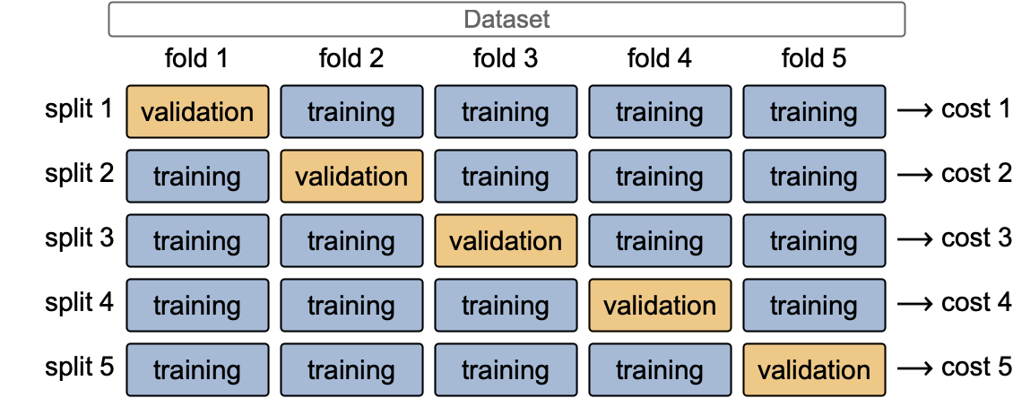
We can then average these cost values to obtain a better estimate of the true validation cost (the one that we would obtain with an infinite validation set). We can use this cross-validation procedure to select the best hyperparameters and then train a model again on the full dataset using these hyperparameters. This kind of cross-validation is called a k-fold cross-validation. We could also generate random training-validation splits, but the advantage of a k-fold cross-validation is that each example is used exactly once as a validation example.
In our polynomial regularization example, there is only one hyperparameter, but this number can be larger. Classic machine learning methods typically have from a few to dozens of them. We can use various global optimization methods to find the best set of hyperparameters. The grid search strategy consists of searching along a grid, and the random search strategy consists of trying a random set of hyperparameters. Here are what these strategies look like for two hyperparameters, λ1 and λ2:
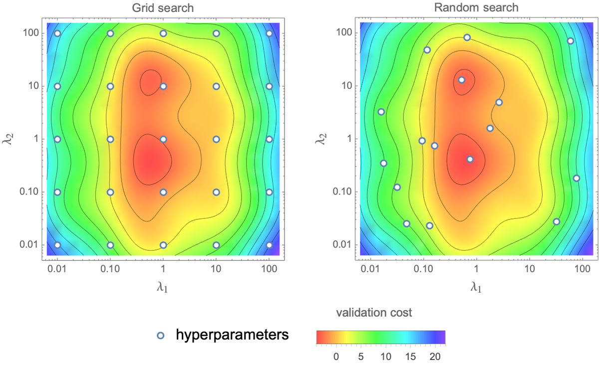
The blue markers are the set of hyperparameters for which the cost is measured, and the background colors indicate the value of the validation cost that we seek to minimize. Random search is typically more efficient than grid search when the number of hyperparameters is larger than 3 or 4.
The automated function Classify adopts a more advanced strategy: it trains many configurations (method + hyperparameters) on small training sets first and then only trains the most promising configurations on larger training sets, which saves time:
Here each curve corresponds to a different method and set of hyperparameters, and we can see that only three configurations have been trained on the full training set.
Another popular way to optimize hyperparameters is to use Bayesian optimization. The idea of Bayesian optimization is to train a cost prediction model from past sets of hyperparameters and to use this model to choose which set of hyperparameters to try next. Typically, the procedure starts by computing the cost for a few random sets of hyperparameters to train a first regression model on this data. The cost prediction model is then used to pick a new promising set of hyperparameters. The cost for this new set is used to train a new cost prediction model and so on. Interestingly, at each step, there is a tradeoff to make between choosing a set of hyperparameters that is most likely to minimize the cost according to the cost model or choosing a set of hyperparameters that is most likely to improve the cost model. This is a classic example of the famous exploration vs. exploitation tradeoff often present in reinforcement learning problems. Note that Bayesian optimization needs a cost prediction model that returns good uncertainties, which is why the Gaussian process method (see Chapter 10, Classic Supervised Learning Methods) is often used for this purpose. The random forest method and even Bayesian neural networks are used as well.
There are plenty of other ways to optimize hyperparameters. Optimizing hyperparameters is an important domain of research that is part of the field of automated machine learning.
It is interesting to think about why we need hyperparameters in the first place and how they are different from regular parameters. Some hyperparameters naturally arise because they correspond to choices that cannot be easily included in the training procedure for technical reasons, such as the connectivity of a neural network. Then there are hyperparameters, like our λ value, that are used for regularization purposes. These regularization hyperparameters cannot be optimized on the training set because it would defeat their purpose (λ would always be 0). Of course, when using automatic functions, hyperparameter optimization is taken care of, so parameters and hyperparameters are merged from this point of view, but even automated functions generally still give the possibility of controlling hyperparameters if desired, which can be used to obtain models more suited to our needs.
Why Predictions Are Not Perfect
Machine learning is a useful tool, but it is not magic, and predictions can be wrong. It is useful to understand the source of model errors in order to improve them. The main sources of errors will be presented in the context of predictive models, but most of these can be transposed to other kinds of models.
Inherent Uncertainty
Generally, the main reason for model errors is just that it is not theoretically possible to make a prediction given the information contained in the input. This type of uncertainty is sometimes called the inherent uncertainty, aleatoric uncertainty, irreducible uncertainty, random noise, or even label noise depending on the context.
For example, let’s say that we want to predict the outcome of flipping an unbiased coin. If we don’t have any information about how the coin is flipped, we cannot do better than making a correct prediction 50% of the time. Even if we had an infinite amount of training examples, we would be constrained by this hard limit. The only way to improve is to obtain additional information, such as the initial velocity of the coin, its distance from the ground, and so on. Without such information, the actual outcome is random from our perspective.
We encountered such inherent uncertainty several times in previous examples. For example, it is intuitively clear that we cannot perfectly predict if a Titanic passenger survived or not solely based on their age, sex, and ticket class:
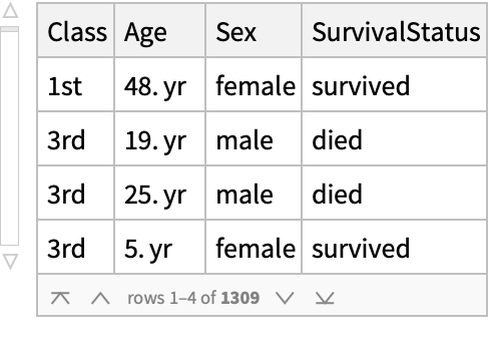
This is confirmed by plotting the accuracy as function of the number of training examples, which seems to saturate around 72%:
The solution to reduce this inherent uncertainty is simply to add informative features. In this case, we would obtain better results if we knew which passengers had children and, of course, if we knew which ones got into a life boat.
Similarly, it is clear that we cannot perfectly predict car stopping distances solely based on their speed. There is too much noise:
The best we can do here is to predict a distribution that aims to represent this uncertainty. Note that this is a justification for the use of probabilistic models.
Inherent uncertainty is not present in every problem though; for example, it is rather small for a classic image identification task:
For this problem, it is theoretically possible to predict the correct class just about every time, at least in its standard formulation. This uncertainty would reappear if the classification was finer grained (more classes) or if images have defects, such as being blurry:
Even the best model cannot know for sure the correct class of such an example.
It is useful to have an estimate of how much inherent uncertainty is present in a given problem in order to set expectations and track the progress of a machine learning project. For the task of classification, the best possible model given current features is called the Bayes classifier, and its error on a test set is called the Bayes error, or irreducible error. For a coin flip, the Bayes error would be 50%. For the Titanic survival problem, without extra information, it should be around 28%. And for a standard image identification problem, it would be closer to 1%. For some applications, such as image identification, we can obtain a good estimate of this error by having humans perform the same task. For other applications, however, this optimal error cannot be obtained from an external system, so we have to resort to using learning curves and guessing what this optimal error might be.
Data Shift
Another origin of error for machine learning models is that training data and in-production data differ too much, which is referred to as data shift. As was explained before, most machine learning methods assume that training data and unseen data come from the same distribution (the iid assumption). This can be somewhat valid, but can also be very wrong. There are various reasons for this.
One reason is that we don’t use good training data in the first place. For example, let’s say that we want to train a model to identify the language of social media messages, such as:
We might train a model on texts from Wikipedia because it is convenient. However, the style and words used on Wikipedia pages are not the same as the ones used on social media. For example, swear words would be completely unknown by this model. This issue is very common. As explained earlier, one partial solution is to diversify the data as much as possible and preprocess it in ways that remove potential differences between training and unseen data.
Another reason is that data changes over time. For our language identification task, this could happen because new words are appearing. For fraudulent transaction detection, this could happen because people use their credit cards differently or because fraudsters adapt to the detection system. This issue is also present in many applications. The remedy here is simply to retrain the model often using recent data. Another thing to keep in mind is that models should be tested on current data instead of past data!
For predictive models, data shifts can be decomposed into two types. The first one concerns in-production inputs that are too different from training inputs. In a sense, this means that these inputs are outliers, which can be defined (although not perfectly) by them being out-of-distribution. Here is an illustration of an out-of-distribution example on Fisher’s Irises data:
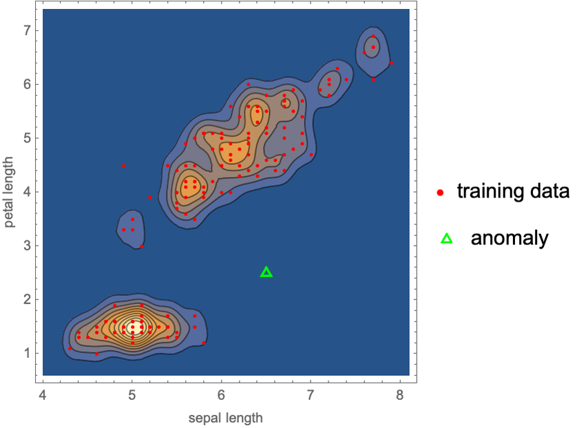
The new example, in green, is clearly not in the same region as the training examples. Such anomalies can sometimes be detected, but this detection task is usually harder than the prediction task itself (see Chapter 7, Dimensionality Reduction, and Chapter 8, Distribution Learning). The alternative is to create models that are good at extrapolating, such as causal models, and are thus more robust, to work on anomalies.
The other type of data shift concerns a change in the relation between inputs and outputs, which means a change in the conditional distribution P (outputinput). This type of change is called a concept drift, and it is not really possible to create models robust to such a change. The solution is thus to detect this type of change, for example, by using good test sets.
It is easy to get fooled by these data shifts, and it is dangerous. We might think our model is performing great because of the measurements on our test sets are good and decide to put the model into production. The results in production will be bad, but we won’t necessarily discover it because we are too confident in our model. For sensitive applications, such as medical diagnostics, the consequences can be significant. To avoid this, it is extremely important to monitor the performance of models in production and to spend even more effort on obtaining a high-quality test set than obtaining a good training set. Since test sets can be much smaller than training sets, it is okay to use slow and expensive techniques to obtain them, such as labeling everything by hand.
Another important problem with data shifts is that they can cause models to be biased against certain groups of people. Let’s say that we use a dataset in which some ethnic groups are underrepresented. Our model might not perform well for people belonging to these groups, which is unfair and might be legally forbidden. This could happen in applications such as facial recognition, medical diagnostics, admission decisions, and so on. These social biases are not only due to training/test differences; they can be introduced in all sorts of ways, even when the creators of the model are cautious about it. Unfortunately, such biased models have been put into production, such as the COMPAS software that in 2016 overestimated the risk of recidivism for black offenders. This issue has been an obstacle to the use of machine learning for such applications. There is an ongoing effort to figure out the best methods and practices to solve these problems, which falls into the domain of responsible AI.
Overall, it is important to be aware of data shift issues, to be skeptical about the performance of models, and to put a lot of effort into creating good test sets.
Lack of Examples
Another common source of errors is simply that we do not have enough training examples. Since machine learning models learn from data, it makes sense that more data leads to better models.
One way to understand this is to consider the simplest possible learning problem. Here we are going to learn the mean of uniform random numbers. Let’s draw 100 numbers between 0 and 1 and compute their mean:
Our result is about 0.48 with a computed statistical uncertainty around 0.03 (which is called the standard error in this case). Let’s now use 1000 numbers instead:
We can see that we are closer to the true value of 0.5 and that the uncertainty is now only about 0.01. This trend continues. Here is what we obtain when changing the number of examples from 100 to one million:
Each time we increase the number of examples by a factor of 10, the uncertainty is reduced by about 3 (the uncertainty scales like ![]() here). In this case, augmenting the number of examples reduces the variance of our estimation, and this is true for just about all machine learning methods. With more examples, we can also increase the complexity of the model to reduce its bias while not necessarily affecting the variance, and thus improving the overall performance.
here). In this case, augmenting the number of examples reduces the variance of our estimation, and this is true for just about all machine learning methods. With more examples, we can also increase the complexity of the model to reduce its bias while not necessarily affecting the variance, and thus improving the overall performance.
An interesting lesson from this simple experiment is that in order to improve a model, it is useless to just add 10% more training examples. We really need to multiply the number by 3 or 10 (notice that the plot is using a log scale). While doing so, it is useful to plot the performance of the model as function of the number of training examples. This is what learning curves are and can be used to estimate how much we would gain by increasing the number of examples further.
Obtaining more training examples can be difficult. For some applications, such as image identification, we can artificially add more examples by performing a data augmentation procedure. We can, for example, blur images, rotate them, distort them, change their colors, etc. Data augmentation can be very efficient. Note that it is an indirect way to add knowledge that we have about the problem.
Another strategy is to add only the most useful training examples. Indeed, rare examples such as “corner cases” typically bring more information than usual examples. Mining such useful examples is a bit of an art, and it breaks the iid assumption made by most machine learning methods, but it can work nevertheless. Active learning (see Chapter 2, Machine Learning Paradigms) is one way to automatically find these useful examples.
Bad Modeling
Finally, the performance of a machine learning model is affected by the modeling process itself, which means the preprocessing, the machine learning method, and the value of the hyperparameters.
Let’s first talk about the preprocessing. When using deep learning methods with a large number of examples, such preprocessing is usually minimal, and the focus is more on the network architecture and connectivity (see Chapter 11, Deep Learning Methods). However, when using classic machine learning methods, which is typically the case on structured data, the preprocessing is a central step in the modeling process (see Chapter 9, Data Preprocessing). The first goal of the preprocessing is to extract good features. Often we have some knowledge about the features that are important, and we should compute them. This is known as feature engineering. Another goal is to remove the irrelevant features and the spurious features. Irrelevant features can statistically hide the relevant features. For example, if we add many random features to a dataset, some of them will be, by chance, well correlated with the output, and the model will use them instead of the relevant features. Similarly spurious features correlate with the output in the training data but not necessarily in unseen data, which might prevent some degree of out-of-distribution generalization.
The choice of method and hyperparameters also affects the quality of the model. One way to interpret this is that machine learning methods make implicit assumptions about the problem (such as a continuity assumption), and we want these assumptions to be suited for the problem at hand. For example, we saw earlier that making “too strong” assumptions (low-capacity model) or “too weak” assumptions (high-capacity model) leads to suboptimal performance. This bias-variance tradeoff is not the only thing to consider. Assumptions are different in nature and some are better than others for a given problem. Here is a conceptual illustration of different assumptions from a Bayesian perspective:
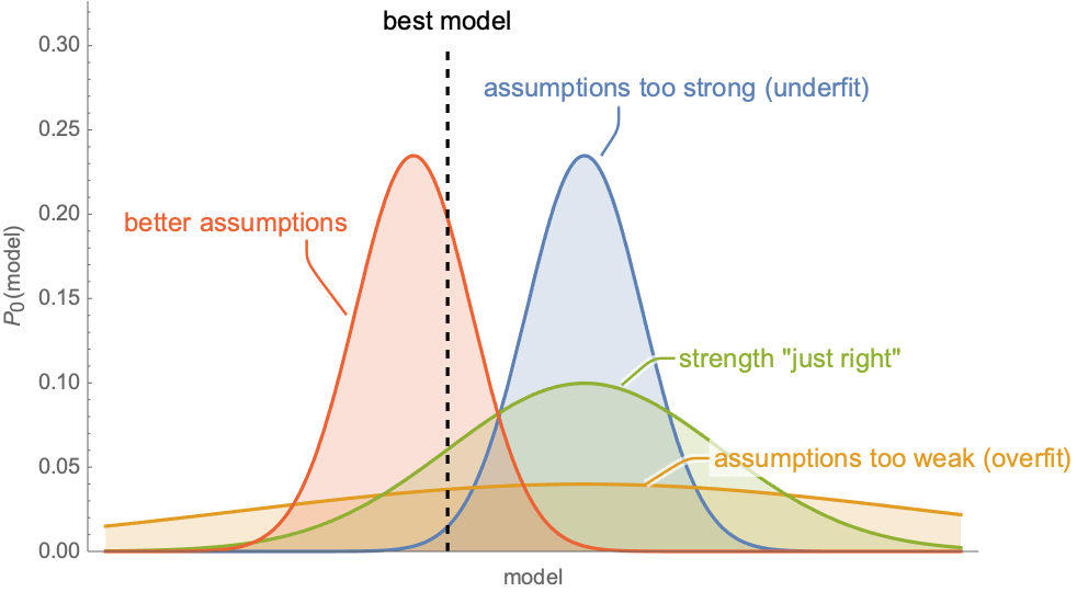
Each curve represents a prior belief over models, which corresponds to our assumptions (see Chapter 12, Bayesian Inference). We can see that relaxing the assumptions represented in the blue curve leads to the green curve, which corresponds to better assumptions (it attributes a higher probability to the best model shown by the dashed line), but using qualitatively better assumptions is even more effective (the red curve).
For problems dealing with structured data, there is a finite set of classic machine learning methods to choose from (see Chapter 10, Classic Supervised Learning Methods). It is relatively easy to try several methods and hyperparameters and see which setting works best on a validation set. Here is the performance of classic methods on the structured dataset ResourceData["Sample Data: Mushroom Classification"]:
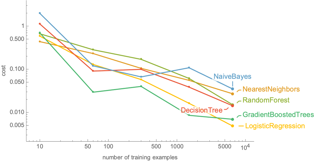
As we can see, selecting the best method leads to substantial improvement for this problem. In other cases, choosing a good method is not that crucial. Overall, these choices can be fairly automatized.
For perception problems, the best models are neural networks. There are plenty of possible network architectures and specific connectivities that we can use, and they perform very differently from each other. As an example, here is the performance of state-of-the-art models (at the time of their release) on the famous ImageNet dataset:
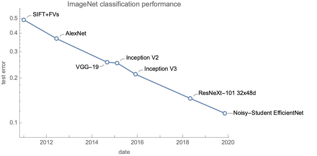
Most of these networks are trained on the same data (except the last two that use extra data), so the main reason for their performance differences is that they use networks that have different connectivity. This shows that for such tasks, the main uncertainty comes from the modeling and not so much from a lack of examples or a lack of information in the input. Note that designing good connectivity from scratch is difficult, so the strategy is usually to reuse an existing network that has been shown to work for similar tasks. An alternative is to automatically search amongst a family of possible architectures (called a neural architecture search), but this is complex and computationally intensive.
| ■ | A model is a mathematical description of a system. |
| ■ | Models are typically described by a formula, a neural network, or a program. |
| ■ | Nonparametric methods make predictions by comparing new examples with training examples. |
| ■ | Parametric methods learn parameters by minimizing a cost function on a training set. |
| ■ | The goal of machine learning models is to generalize to unseen data. |
| ■ | Model capacity can be tuned to improve performance. |
| ■ | Hyperparameters are the values that need to be set before the training process. |
| ■ | Good hyperparameters can be obtained through a validation procedure. |
| ■ | Some machine learning methods work better than others for a given problem. |
| ■ | Better features and more training examples generally improve the quality of a model. |
| ■ | It is easy to get fooled into believing a model is good. |
| ■ | Effort should be put into creating good test sets. |
| parametric methods | machine learning methods that generate models defined by a fixed set of parameters | |
| parameters | values that uniquely define a model | |
| model family | collection of possible models | |
| nonparametric methods | machine learning methods whose model size varies depending on the size of the training data | |
| instance-based models memory-based models neighbor-based models similarity-based models | models that make predictions by finding similar examples in the training set | |
| optimization | process of searching a configuration (here, a model) that maximizes or minimizes a given objective | |
| cost function empirical risk objective function | model measure that is optimized during the training phase | |
| loss function | per-example model measure that is used to compute the cost/risk/objective function | |
| squared error loss quadratic loss | usual regression loss, squared deviation from the truth for a given example | |
| cross-entropy loss log loss | usual classification loss, logarithm of the correct-class probability for a given example | |
| feature vector | set of numeric features representing an example | |
| feature engineering | creating good features manually | |
| neural architecture search | automatic search for new neural network architectures | |
| nearest neighbors | machine learning method that makes predictions according to the nearest examples of the training set | |
| linear regression | machine learning regression method that predicts a numeric value by performing a linear combination of the features | |
| logistic regression | machine learning classification method that predicts class probabilities using a linear combination of the features |
| model generalization | ability for a model to work correctly on unseen data | |
| unseen data | data that was not in the training set | |
| iid assumption | the assumption that all data examples come from the same underlying distribution and have been sampled independently from each other (independently and identically distributed) | |
| in-distribution example in-domain example | data example that comes from the same underlying distribution as the training examples | |
| out-of-distribution example out-of-domain example | data example that comes from a different underlying distribution than the training examples (similar to an anomaly or an outlier) | |
| in-distribution generalization | ability of a model to work correctly on unseen examples that come from the same distribution as the training examples | |
| out-of-distribution generalization | ability of a model to work correctly on examples that come from a different distribution than the training examples | |
| robust model | model that works well for a wide range of data examples, such as out-of-distribution examples | |
| brittle model | model that only works well for a narrow range of data examples, such as only in-distribution examples | |
| irrelevant features | features that do not bring information about the meaning of the data example | |
| spurious features | features that capture the meaning of training data examples but not the meaning of new data examples (because of a data shift) | |
| semantic features | features that capture the meaning of all data examples | |
| learning bias inductive bias prior knowledge prior hypotheses | assumptions made by a machine learning method about the data in order to learn models that generalize | |
| model fit | how well a model matches the data | |
| model capacity | ability of a model family to fit the various data it is trained on | |
| underfitting regime | when the capacity of a model family should be increased in order to obtain models that generalize better | |
| overfitting regime | when the capacity of a model family should be decreased in order to obtain models that generalize better | |
| validation set development set | dataset used to measure the performance of a model during the modeling process (for example, to compare candidate models) | |
| test set | dataset used to measure the performance of a model after the modeling process to obtain an unbiased estimation of the performance | |
| bias-variance tradeoff | generalization tradeoff between the model bias (amount of assumptions made by the model) and model variance (sensitivity of the model to the training data), tradeoff made by changing the model capacity |
| regularization smoothing | process of the controlling of the capacity of a model family | |
| hyperparameter | all of the parameters of a machine learning method that are not learned during the training procedure and thus need to be set before training | |
| L2 regularization L2 penalty | classic regularization strategy for parametric models, penalize large parameters in the cost function | |
| early stopping | classic regularization strategy for neural networks, stops the training when the validation cost does not decrease anymore | |
| cross-validation | model evaluation procedure that consists of training and testing a model several times on different training-validation splits of the dataset | |
| k-fold cross-validation | cross-validation technique that consists of creating k training-validation pairs by splitting the dataset into k intervals of the same size | |
| grid search | optimization method that searches along a grid, used for hyperparameter optimization | |
| random search | optimization method that searches randomly, used for hyperparameter optimization | |
| Bayesian optimization | optimization method that uses a model trained on past attempts to predict where the optimum is, used for hyperparameter optimization | |
| exploration vs. exploitation tradeoff | tradeoff between exploring new areas in order to learn further or making use of what we already know, typically present in reinforcement learning and optimization problems | |
| automated machine learning | machine learning for which hyperparameter/model selection and preprocessing steps are automatic |
| inherent uncertainty aleatoric uncertainty irreducible uncertainty random noise label noise | uncertainty on the predicted label value stemming from a lack of information in the input | |
| Bayes classifier | classifier whose prediction uncertainty is irreducible, best possible classifier given the features | |
| Bayes error irreducible error | test error for the Bayes classifier | |
| data shift | difference between training data and in-production data | |
| concept drift | change in the relation between inputs and outputs in production data | |
| social bias | bias against a group of people sharing some characteristics (such as age, gender, disability, or ethnicity) that is considered to be unfair | |
| responsible AI | set of methods and practices aiming to build ethical machine learning models, the main focuses are on fairness, interpretability, privacy, security, and accountability |