Dimensionality reduction is another classic unsupervised learning task. As its name indicates, the goal of dimensionality reduction is to reduce the dimension of a dataset, which means reducing the number of variables in order to obtain a useful compressed representation of each example. We can interpret this task as finding a lower-dimensional manifold on which the data lies or as finding the latent variables of the process that generated the data. Dimensionality reduction is the main component of feature extraction (also called feature learning or representation learning), which can be used as a preprocessing step for just about any machine learning application. Dimensionality reduction can also be used by itself for specific applications such as visualizing data, synthesizing missing values, detecting anomalies, or denoising data.
In the first section of this chapter, the concept of dimensionality reduction will be introduced, and in the other sections, we will explore various applications of this task. While dimensionality reduction can be a supervised learning task, it is generally unsupervised. All of the examples in this chapter are unsupervised.
Manifold Learning
Let’s start by creating a simple two-dimensional dataset in order to understand the basics of dimensionality reduction and its applications:
We can see that the data points are not spread everywhere; they lie near a curve. This is not surprising because we explicitly constructed the data to follow (up to some noise) a parametric curve defined by:
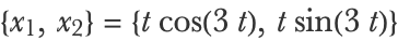
Here x1 and x2 are two features and t is the parameter that can be changed to obtain the curve. This curve on which the data lies is called the manifold of the data. Dimensionality reduction is the task of discovering such a parametrized manifold through a learning process. Once learned, the manifold can then be used to represent each data example by their corresponding “manifold coordinates” (such as the value of the parameter t here) instead of the original coordinates ({x1,x2} here). These manifold coordinates can be seen as the latent variables of a process that generated the data, and since the number of coordinates is reduced (from 2 to 1 here), it is called a dimensionality reduction.
Let’s attempt to discover such manifold and latent variables using the classic Isomap method:
The output is a function that can be used to reduce the dimension of new data, for example:
It is also possible to go in the other direction and recover the original data from reduced data:
We can see that the reconstructed data is not perfect; there is a loss of information in the reduction process.
To better understand what is going on, let’s visualize the learned manifold. We can do this by inverting the reduction for several reduced values (going from several instances of t to their corresponding {x1,x2}):
We can see that the learned manifold is close to the original manifold, but they are different since the learned manifold is just a model. Also, the result is not smooth because the Isomap method uses a nonparametric model. There are also parametric methods to perform dimensionality reduction, the most classic one being principal component analysis (PCA). Let’s now visualize the reduced values on the manifold using colors:
We can see that along the manifold, the reduced values range from -4.5 (in red) to 3 (in blue). Note that these values are different from our original parameter t that ranges from 0 to 1. This is normal. There is nothing special about the original parametric curve; many equally valid parametric curves could be defined (e.g. by shifting or scaling the parameter).
In this plot, we also show where each data point belongs on the manifold. We can see the reduction process as a kind of projection of the data on the manifold. More precisely, the dimension reducer defines a mapping from the entire space to the manifold. This explains why the information is not preserved perfectly: only data points that lie exactly on the manifold are perfectly encoded. Data points that are not on the manifold have an imperfect encoding, but since the data is supposed to be near the manifold, most of the information should be preserved. This loss of information can be quantified by a reconstruction error, which is the mean squared Euclidean distance between the data and reconstructed data (i.e. projected on the manifold):
We should, however, compute this value using a test set since the reducer, like any other machine learning model, tends to perform better on the training data than on unseen data. Let’s compute the reconstruction error over 1000 test examples:
A perfect value here would be 0. This value can be compared to the overall variance of the data that constitutes a baseline (this would be the reconstruction error if the manifold was a unique point at the center of the data):
In this case, the reconstruction error is much smaller than the baseline, which makes sense since we can see that the data lies close to the learned manifold. The reconstruction error is the usual way to compare dimensionality reducers in order to select the best one. It is not a perfect metric though, as we might care about something other than a Euclidean distance for some applications (e.g. various semantic distances). Also, such an error is hard to compare when the reduced dimensions of the models are not the same (do we prefer to divide the dimensions by 2 or the reconstruction error by 2?). There are some heuristics to pick an appropriate dimension, but there is not a perfect metric for that. It really depends on the application, like for choosing the number of clusters in clustering.
In a sense, dimensionality reduction is the process of modeling where the data lies using a manifold. This knowledge of where the data lies is pretty useful, for example, to detect anomalies. Let’s define and visualize the anomalous example {x1,x2}={-0.2,0.3} along with its projection on the manifold:
Taken by themselves, x1=-0.2 and x2=0.3 are perfectly reasonable values. Taken together though, we can see that the anomaly, or outlier, is far from the other data points. This manifold offers us a way to quantify how far an example is from the rest of the data by computing the distance of the example to its projection on the manifold, which is its reconstruction error:
In this case, the reconstruction error is 0.085, which is much higher than the average error (about 0.003), so we can conclude that the example is anomalous. Dimensionality reduction models can therefore be used as anomaly detectors by simply setting a threshold on the reconstruction error.
Another application of knowing where the data lies is denoising, or error correction. A noisy/erroneous example is a regular example that has been modified in some way (a.k.a. corrupted) and is now an outlier. In order to “de-outlierize” the example, we can project it on the manifold and obtain a valid denoised/corrected example. Here is what it would give for our anomaly:
One advantage of using such a method to denoise is that we do not assume much about the kind of noise/error that we are going to correct, which makes it robust. However, when the type of noise is known beforehand, we can obtain better performance by training models in a supervised way to remove this specific noise using methods such as a denoising autoencoder.
Finally, knowing where the data lies can be used to fill in missing values, a task known in statistics as imputation. Let’s say that we know that x1=-0.6 but that x2 is unknown. We can compute the intersection of the line defined by x1=-0.6 and the manifold, which is where the data is most likely to be. This would give us x2≃0.47:
If there is no intersection (for example, when x1=0.3), we can just find the point that is the closest to the manifold, which means minimizing the reconstruction error. If there are several intersections, on the other hand, we have several possible imputation values. In Chapter 8, Distribution Learning, we will see how to fill in missing values in a more principled way.
Detecting anomalies, filling in missing values, and denoising are common applications of dimensionality reduction. However, the main application of dimensionality reduction is probably to preprocess data for a downstream machine learning task such as clustering, classification, or information retrieval (search engines). There are a number of reasons why we would want to reduce the dimension as a preprocessing step. In classification, for example, it can be useful if many labels are missing (a setting known as semi-supervised learning—see Chapter 2, Machine Learning Paradigms), or if the data is very unbalanced (which means that some classes have a lot fewer examples than others), or sometimes just as a regularization procedure.
It is interesting to think, in a more philosophical sense, about why dimensionality reduction is useful at all. In our two-dimensional case, by discovering the manifold on which the data lies, we removed part of the noise. This means that the data is more informative and is easier to learn from. Now, in a more general view, real data (especially high-dimensional data) always lies in a very thin region of their space (which, in practice, is not necessarily a unique continuous manifold but rather a multitude of manifolds). A good example is the case of images. Real-life images never look like a random image:
Rather, real images have uniform regions, shapes, recognizable objects, and so on:

This means that images could theoretically be described using a lot fewer variables. Instead of pixels, we could use concepts such as “there is a blue sky, a mountain, a river, and trees at such and such positions,” which is a more compressed and semantically richer representation. The interesting thing is that learning to describe images with a small number of variables forces you to invent such semantic concepts (not necessarily the same as human concepts though). So in a very broad view, dimensionality reduction is a process for understanding the data by inventing a numeric language in which data examples can be simply represented. Once such a representation is found, just about every downstream task is easier to tackle because the understanding is already there. The drawback is that the reduction is unsupervised and thus, like for clustering, the goal is not well defined. This means that there is a chance that the resulting numeric language is not really the one we are interested in for our application or downstream task. Choosing appropriate features, distances, and algorithms is often necessary.
Data Visualization
One straightforward application of dimensionality reduction is dataset visualization. The idea is to reduce the dimension of a dataset to 2 or 3 and to visualize the data in this learned feature space (a.k.a. latent space). This technique is heavily used to explore and understand datasets. Let’s use 1000 images of handwritten digits to illustrate this:
In order to visualize this dataset, we reduce the dimension of each image from 728 pixel values to two features and then use these features as coordinates for placing each image:
As expected, digits that are most similar end up next to each other. Such a feature-space plot helps us understand the data. For example, we can see that there are clusters that correspond to particular digits. We can also see how these clusters are organized, and we can spot potential anomalous examples around the cluster borders. Overall, we get a feel for what the dataset is and how it is structured. This plot is obtained by using a dimensionality reduction method specialized for visualizations (called t-SNE here). Of course, such a drastic dimensionality reduction (from 728 pixel values to only two values) leads to an important loss of information. The data is pretty far from the learned manifold, but it does not matter much for visualization.
Let’s now create feature-space plots on a subset of the images that we used in Chapter 3:
First, let’s apply the dimensionality reduction directly to pixel values:
We can see that the images are grouped according to their overall color. For example, images with dark backgrounds are on the top-left side while bright images are on the bottom-right side. The semantics of the image, such as mushroom species, is ignored. This is not surprising given that the reduction only has access to pixel values and that the number of images is too small to learn anything semantic. With a lot more images and more computation, it could be possible to discover such semantic features and obtain a more useful plot. Nevertheless, we are faced with the same problem as in the clustering case: the computer does not really know our goal. We could want things to be grouped according to their type, their color, or their function, and so on. Again, we can use a specific feature extractor to guide the process, such as using features from an image identification neural network:
We can now see much more semantic organization: mushrooms of the same species are clustered together while background colors are largely ignored. This plot also helps us understand why our classifier was so successful: species are pretty much identified even without labels thanks to this feature extractor.
Feature-space plots are not limited to images. Here is an example using the Boston Homes dataset (only a few variables are displayed here):
Again, we can see clusters, which we should analyze further to see what they correspond to. It would be interesting to see if they correspond to actual districts (and if their positions on the plot somewhat correspond to their geographic locations, which can happen with such data).
Feature-space plots are generally two-dimensional, but they can also be three-dimensional, which gives more room for including additional structures and relations between examples. Overall, feature-space plots are excellent tools for exploring datasets and are heavily used nowadays, probably even more than hierarchical clustering (which serves a similar purpose).
Search
Being able to obtain a vector of latent variables for each example is very useful for searching a database. One straightforward reason is that it is easy to define a distance on numeric vectors. More importantly, using reduced vectors speeds up the search process and can lead to better search results. Let’s illustrate this by constructing a synthetic database using a book. We first load The Adventures of Tom Sawyer and split it into sentences:
Here is a random sentence from this book:
Each sentence corresponds to a document in our fictional database. In order to reduce the dimension of each document, we first need to convert them into vectors. This can be done by segmenting the text into words and then computing the tf–idf vectors of these documents (see Chapter 9, Data Preprocessing):
tf–idf is a classic transformation in the field of information retrieval that consists of computing the frequency of every word in each document and weighting these words depending of their rarity in the dataset. The corresponding feature extractor generates a sparse vector of length 8189 (the size of the vocabulary in the dataset):
Since we can convert each sentence into a vector, we can now compare sentences easily using something like a cosine distance:
The problem is that the distance computation took 0.1 milliseconds, which can become prohibitively slow for searching a large dataset. To improve this, let’s reduce the dimension of the dataset to 50 features:
Computing a distance between vectors of this size is at least 10 times faster that before, and we can preprocess the dataset beforehand. For a large-scale search engine, such a dimensionality reduction procedure can be pushed to the extreme by reducing each example to 64 Boolean values, which means we can store each vector using a 64-bit memory address. This is called semantic hashing and makes searching extremely fast.
Let’s now create a function that finds the nearest example in this reduced space:
This function acts like a search engine. We can give it a query and it will return its nearest elements in the dataset. Here are the two nearest sentences for a given query:
Speed is critical for search engines, which is why such dimensionality reductions are necessary. But speed is not the only benefit of this procedure: the manifold can capture semantic concepts in the data, so the distance along the manifold is generally better (depending on our purpose) than the distance in the original space. In that case, it seems to be true. Here are the two nearest sentences found without using the dimensionality reduction:
Anomaly Detection & Denoising
Let’s now use a high-dimensional dataset to illustrate how we can detect anomalies and denoise data using dimensionality reduction. Let’s again use the handwritten digit images from the classic MNIST dataset:
Let’s create a training set of 50000 examples and a test set of 10000 examples:
To make things simpler (notably to handle missing values), we will work with arrays instead of images. Here are functions to convert an image into a numeric vector and a vector back to an image:
Each image corresponds to a vector of 28×28=784 values. Let’s convert one image into a vector:
Let’s now train a model on the training set to reduce the data to 50 dimensions:
As expected, the reducer produces 50 values from a vector of size 728:
This reducer corresponds to a manifold on which the data approximatively lies. Let’s see if it can be used to detect anomalies. Here are three examples from the test set:
Let’s project these examples on the manifold:
We can see that the reconstructions are not perfect but still somewhat close to the original examples. Let’s compute their reconstruction errors:
These errors all are between 10 and 20. Let’s now define anomalous examples using a random image, an image of a face, and corrupted versions of our test examples:
Again, we can visualize their projections on the manifold:
We can see that these reconstructions are not as good as before, especially the first three that are particularly bad. Let’s see if this translates into high reconstruction errors:
The reconstruction errors for the first three examples (![]() ,
, ![]() , and
, and ![]() ) are more than 1000 higher than errors for the test examples. This means that we can easily set a threshold on the reconstruction error to identify such anomalies. Example
) are more than 1000 higher than errors for the test examples. This means that we can easily set a threshold on the reconstruction error to identify such anomalies. Example ![]() has a somewhat higher reconstruction error, so it could be identifiable as well. The other examples(
has a somewhat higher reconstruction error, so it could be identifiable as well. The other examples(![]() and
and ![]() ), however, have a good reconstruction error, which means that they are too close to the learned manifold to be detected as anomalies. We can clearly see that these images are anomalies though. Our model is just not good enough to detect them.
), however, have a good reconstruction error, which means that they are too close to the learned manifold to be detected as anomalies. We can clearly see that these images are anomalies though. Our model is just not good enough to detect them.
Let’s now see if we can denoise the data. The process simply consists of projecting the data on the manifold. Here are the corrupted images and their “corrections” side by side:
The results are pretty bad, except for the jittered image (![]() ) for which the corrected version is acceptable (
) for which the corrected version is acceptable (![]() ). Again, this shows that our model is not perfect, but it also shows the limitation of error correction using a fully unsupervised approach and therefore being noise agnostic. We would probably obtain better results by training a model in a supervised way to denoise these specific kinds of noises.
). Again, this shows that our model is not perfect, but it also shows the limitation of error correction using a fully unsupervised approach and therefore being noise agnostic. We would probably obtain better results by training a model in a supervised way to denoise these specific kinds of noises.
Missing Data Synthesis
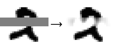
Let’s now try to synthesize (a.k.a. impute) missing values using the same handwritten digits. We introduce missing values in the test examples by replacing pixels of lines 10 to 15 with missing values:
Let’s visualize the resulting images by coloring the missing values in gray:
We want to replace missing values with plausible numbers. To do so, we need to generate images that are close to the manifold and for which the known values are identical to the original images. We thus need to minimize the reconstruction error while keeping the known values fixed. We could use various optimization procedures for that. Here let’s use a simple yet efficient method: we start with a naive imputation (all pixels replaced with gray), then project on the manifold, then replace the known values of the projection by what they should be, and then project again. If we repeat this process several times, we should get close to the manifold while keeping the known values fixed. Here are 40 iterations of this procedure on a test example:
The imputation procedure seems to work. The missing pixels are gradually replaced with colors that make sense given the training data. The final image seems plausible (still not perfect though):
We should stress that our imputer knew nothing about images in general; it learned everything from the training set. This also means that this imputer can only work on similar images.
Autoencoder
In the previous sections, we used automatic functions to reduce the dimension of the data. Let’s see how we can use a neural network to perform this task. The advantage of using a neural network is that we can tailor the architecture of the network to better suit our dataset, which is particularly useful in the case of images, audio, and text (see Chapter 11, Deep Learning Methods).
Let’s continue using the MNIST dataset, which we split into a training set and a test set:
To reduce the dimension of this data, we are going to use an autoencoder network. An autoencoder is a network that models the identity function but with an information bottleneck in the middle. Here is an illustration of a fully connected autoencoder:
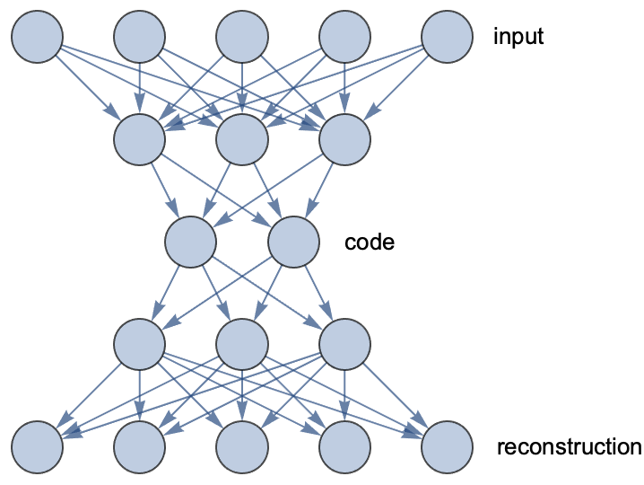
This network gradually reduces the dimension from 5 to 2 and then increases the dimension back to 5. Such a network is trained so that its output is as close as possible to its input, which forces the network to learn a compressed representation (the code) at the bottleneck. The first part of this network is called an encoder, and the second part is called a decoder.
Let’s implement an autoencoder for our handwritten digits:
This network progressively reduces the dimensions from 784 values (the number of pixels) to 30 values and then back to 784 values to recreate an image. This is a self-normalizing architecture (see Chapter 11, Deep Learning Methods). Currently this network is not trained, so the reconstructed image is random:
To train this network, we need to attach a loss that compares the input and the output, such as using the mean square of pixel differences:
Let’s train this network on our training set:
The validation curve is going down, which is what we want. We would even gain from training this network for a longer time. Notice that the validation cost is, strangely, lower than the training cost. This is just an artifact created by the dropout layers that behave differently at training and evaluation time (explained in Chapter 11, Deep Learning Methods). Let’s extract the trained network:
To use this autoencoder as a dimensionality reducer, we need to extract its encoder part:
We can now convert any input into its vector representation:
We can also use the entire autoencoder to reconstruct images:
Let’s try this network on an example:
As we can see, the reconstruction is now close to the original input. Let’s see if we can denoise images with this autoencoder:
The results are quite a bit better than for our previous attempt at this problem but not quite perfect yet. To obtain better results, we could try to train longer using a bigger model or using a convolution architecture (see Chapter 11, Deep Learning Methods). Now, if we only want this network to work well for a particular kind of noise, an even better strategy is to train it in a supervised way to remove this particular noise. For example, the data could look like:
The resulting model is called a denoising autoencoder (and it does not necessarily need a bottleneck anymore). Training a denoising autoencoder is also a method to teach a vector representation in a supervised way (or rather, a self-supervised way).
Recommendation
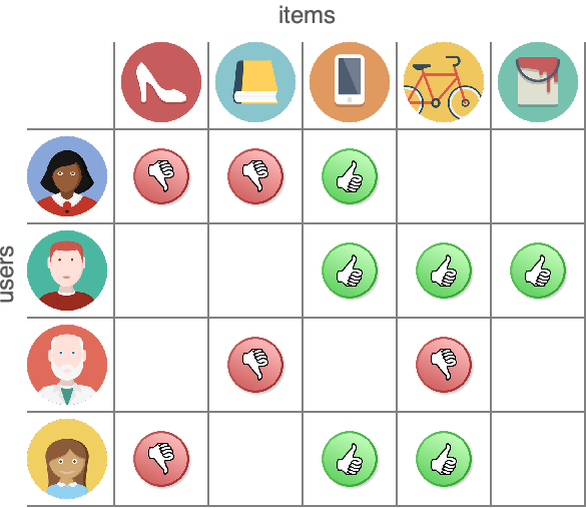
Recommendation (and more generally content selection or content filtering) is the task of recommending products, books, movies, etc. to some users. Such a task is extremely common for e-commerce but is also used by social media to choose which content to display. In practice, recommendation is a messy business and many methods can be used depending on the situation. Here we will focus on an idealized collaborative filtering problem, which means figuring out the preference of a user based on everyone else’s preference.
We have a set of users who rated items according to their preference. Ratings could be “like” vs. “dislike” or a number between 1 and 5, for example. The data is usually set up as a matrix where rows are users and columns are items:
Let’s use a dataset of 100 users who rated 200 movies (extracted from the MovieLens dataset):
Ratings are numbers between 0.5 and 5:
Let’s visualize this matrix (missing values are replaced with 0):
The data is sparse, with a density of around 6%, which means that most ratings are missing because users have probably not seen these movies.
The goal is to predict which movie a user would prefer amongst their unseen movies. One way to achieve this is to predict the ratings that the user would give to all movies and then to select the highest-rated movies. In other terms, we need to fill in the missing values of the matrix. We saw in the previous section that it is possible to fill in missing values using dimensionality reducers. The problem is that our training data already has missing values. It is a bit of a chicken-and-egg problem. One naive solution could be to fill in missing values randomly, then train a reducer, then fill in missing values using the reducer, and repeat this process until convergence, as we did for the handwritten digits (see the Missing Data Synthesis section in this chapter). This self-training procedure is a variant of the expectation-maximization algorithm normally used to teach distributions (see Chapter 8, Distribution Learning) and can be efficient, but it would not work well in our case because there are too many missing values.
As it happens, some dimensionality reduction methods (such as low-rank matrix factorization but also autoencoders) are able to learn from training sets that have missing values by simply minimizing the reconstruction error on the known values, so we will use one of these methods. But first, let’s preprocess the data a little bit. Since we know that ratings have to be between 0.5 and 5, we use logit preprocessing so that new ratings can take any value:
This will constrain any prediction into the correct range. Let’s now train a reducer with a target dimension of 10:
We can now use this reducer to predict the ratings of any user. Let’s apply it to the first 10 movies for the first user:
The second prediction is the highest here, so amongst these 10 movies, we would recommend the second one. We can also visualize the full matrix imputed by the predictions:
In order to assess the performance of this predictor, we should use a test set and compare some predictions with their real ratings.
It is interesting to think that we can predict movie ratings without any information about the movies or users. This is possible because for each user, there is a corresponding set of users that have similar preferences (given enough data). In a way, the problem is to identify such a set of similar users. What is happening here is that our reducer knows where the users are in this movie-rating space (they are on the learned manifold). Given ratings from a specific user, the reducer can figure out the most likely position of this user in this rating space (by minimizing the reconstruction error) and thus obtain all of their preferences.
One difficulty of the recommendation task is that there is a feedback loop: current recommendations influence future data, which in turn influences future recommendation systems. Because of this feedback loop, a recommendation system can get stuck into recommending the same kind of things while ignoring other good content. One easy solution is to add noise to obtain a higher diversity. A more complex solution is to treat recommendation as a reinforcement learning problem, which is what this task really is.
Another issue with recommendation systems is that they can have unintended consequences on users, especially in the context of social media. For example, a “too good” recommendation system might make users addicted or always provide engaging but extreme content. Besides obvious ethical issues, these problems might also lead users to eventually stop using the product given the long-term negative impact it has on their life. There is no easy solution to solve this besides adding side objectives (more content diversity, down-weighting extreme content, etc.) or giving the possibility for users to personalize the recommendation engine in some way.
| ■ | Dimensionality reduction is the task of reducing the number of variables in a dataset. |
| ■ | Dimensionality reduction can be interpreted as finding a parametrized manifold on which the data lies. |
| ■ | Dimensionality reduction can be interpreted as finding the latent variables of the data-generating process. |
| ■ | Dimensionality reduction can be useful as a preprocessing step for just about any downstream task. |
| ■ | Dimensionality reduction can be used to visualize data, fill in missing values, find anomalies, or create search systems. |
| ■ | Like clustering, dimensionality reduction cannot be as automated as supervised learning tasks and thus requires more work from the practitioner. |
| dimensionality reduction | task of reducing the number of variables in a dataset | |
| feature extraction feature learning representation learning | task of learning a useful set of features to represent data examples | |
| manifold | hypersurface meant to represent where the data lies | |
| latent variables | unobserved variables that are part of the data-generating process | |
| feature space latent space | space of features after the dimensionality reduction | |
| feature-space plot | plot displaying the examples of a dataset in their 2D or 3D learned feature space | |
| parametric curve parametric surface | curve/surface where each coordinate is a function of some latent variables (called parameters here) | |
| reconstruction error | measure of the quality of a dimensionality reduction, mean squared Euclidean distance between the data and reconstructed (reduction + inverse reduction) data | |
| anomaly outlier | data example that substantially differs from other data examples | |
| anomaly detection | task of identifying examples that are anomalous | |
| denoising error correction | task of removing noise or errors in data examples | |
| information retrieval search | task of retrieving information in a collection of resources | |
| imputation missing data synthesis | task of synthesizing the missing values of a dataset | |
| semantic hashing | dimensionality reduction that maps examples to Boolean vectors representing computer memory addresses | |
| recommendation content selection content filtering | task of recommending products, books, movies, etc. to some users | |
| collaborative filtering | figuring out the preference of users based on everyone else’s preferences | |
| autoencoder | a neural network that models the identity function but with an information bottleneck in the middle, consists of an encoder and a decoder part | |
| encoder | a neural network that encodes data examples into an intermediary representation | |
| decoder | a neural network that uses an intermediary representation to perform a task | |
| denoising autoencoder | a neural network trained in a supervised way to denoise data | |
| principal component analysis | classic method to perform a linear dimensionality reduction, finds the orthonormal basis, which preserves the variance of the data as much as possible | |
| low-rank matrix factorization | classic method to perform a linear dimensionality reduction, approximates the dataset by a product of two (skinnier) matrices | |
| Isomap | classic nonlinear dimensionality reduction method, attempts to find a low-dimensional embedding of data via a transformation that preserves geodesic distances in a nearest neighbors graph |