Let’s explore further the task of classification, which is arguably the most common machine learning task. Classification is a supervised learning task for which the goal is to predict to which class an example belongs. A class is just a named label such as "dog", "cat", or "tree". Classification is the basis of many applications, such as detecting if an email is spam or not, identifying images, or diagnosing diseases. This task will be introduced by training and using classifiers on a few problems.
Car vs. Truck
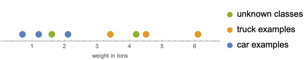
To understand the classification task better, let’s consider this minimal (and artificial) dataset for which the goal is to predict if a vehicle is a car or a truck based on its weight in tons:
Each of these six examples is an input-output pair for which the input is a numeric value (the weight) and the output is a class that can be either "car" or "truck". Let’s visualize these examples in their input space:
We want to learn from these examples how to classify new input values, such as a weight of 1.6 tons or 4.2 tons. Because there are exactly two classes in the training set, this is called a binary classification problem. In order to achieve this, we can use the automatic machine learning function Classify on the dataset:
Classify used the data in order to return a classifier, which is a program that is able to classify new examples. We can give any new weight to the classifier to obtain a class. For example, a weight of 1.6 tons is classified as a car:
And a weight of 4.2 tons is classified as a truck:
These classifications make sense if we look at the training data because vehicles with weights around 1.6 tons are cars while vehicles with weights around 4.2 tons are trucks:
The situation is more ambiguous for a weight of 2.7 tons:
For such examples, it is useful to know the confidence that the classifier has in its decision. This can be obtained by asking the classifier to return a probability for each class:
These class probabilities can be interpreted as the “belief” of the classifier. In this case, the classifier thinks that a vehicle that weights 2.7 tons has about 60% chance of being a car and about a 40% chance of being a truck. As expected, the classifier is much more confident when the weight is 1.6 tons:
Most machine learning models can return probabilities (or at least a score that can be transformed into a probability). Such models are said to be probabilistic. Probabilities are useful in deciding if the classification can be trusted or if an alternative treatment should be considered (see the section From Probabilities to Decisions in this chapter for more details). Let’s visualize the probabilities of our classifier for each possible input value:
We can see that the classifier is confident that weights smaller than ~2.5 tons correspond to cars and that weights larger than ~3 tons correspond to trucks. Between 2.5 and 3 tons, the classifier is not so sure, and its decision switches from car to truck around 2.76 tons, which is called a decision boundary:
Note that class probabilities sum to 1. This means that the classifier returns either "car" or "truck", but never “none of them” nor “both of them.” One way to return “none of them” could be by setting a probability threshold (e.g. 90%) under which no class is returned. Another way is to train a specific anomaly detection model (see Chapter 7, Dimensionality Reduction, and Chapter 8, Distribution Learning) that rejects any input that is not similar to the training inputs. In order to return “both of them,” however, one would need to train a multi-label classifier, which independently predicts the presence/absence of every possible class, and this is another kind of classifier altogether.
Titanic Survival
Let’s now perform a similar analysis on a more realistic (yet still quite simple) dataset. We will use a dataset of 1309 Titanic passengers for which their class, age, sex, and survival status have been recorded:
This is an example of structured data, and, more particularly, of tabular data since the data is a table. Each row corresponds to an example, and each column corresponds to a different variable. Variables of tabular data are generally numbers and classes, although they can also be dates, text, etc. In this case, there are four variables. One of them ("Age") is a numeric variable because its values are numbers or numeric quantities. The three other variables ("Class", "Sex", and "SurvivalStatus") are nominal variables, also known as categorical variables. The values of nominal variables are classes, which also means that we can train a classifier to predict any of them.
Before creating a classifier, let’s analyze the data further. Exploratory data analysis is an important first step of every machine learning project, at least to check that everything looks right. The first thing to notice is that the variable "Age" contains about 20% missing values:
Many datasets have missing values. When using automatic tools, this should not be a problem. Without such tools, however, or to do a finer-grained modeling, this should be addressed in some way (see Chapter 7, Dimensionality Reduction, and Chapter 8, Distribution Learning). Let’s visualize a histogram of the non-missing values:
Everything looks fine. There are no negative or exceedingly high ages and the data does not seem long-tailed (i.e. spanning many orders of magnitude). So far so good. Let’s now analyze the nominal variables using pie charts:
We can confirm that these variables are nominal, there are no missing values, and there are no obvious errors either. We could train a classifier to predict any of these variables, but let’s choose to predict the survival status. The possible classes are "survived" and "died" (again a binary classification problem), and we can see that their frequency is similar (about 60% died), so the dataset is said to be balanced. Datasets with very different class counts (ratios at least higher than 10) are said to be imbalanced and can require special treatment.
Things are looking good for this dataset. There isn’t much preprocessing to do. Let’s move on to the training phase. First, we extract the features from the dataset:
Then we extract the classes:
Now we can train a classifier to predict the classes as function of the features:
Note that we told the function to spend about one second and to use the "RandomForest" method, which corresponds to a specific kind of model. Since Classify is an automated function, it is not necessary to give such specification, but it can be useful if we already know which model would perform best on our data. In Chapter 10, Classic Supervised Learning Methods, we will look at what these models are.
Let’s try the classifier on new examples. A young female traveling in first class would likely survive:
On the contrary, an older male in third class would probably die:
Sometimes we want an explanation for such predictions in order to know if we can trust them. There is no perfect way to explain a prediction, but there are methods to assign an importance value to each feature. A popular one is called SHAP, which stands for Shapley additive explanations. The idea of SHAP is to compare model predictions with and without the presence of a feature to estimate its influence. Here are the SHAP values explaining why the young female traveling in first class survived:
Being a female triples the odds of surviving for this passenger (the odds of an event is ![]() , where p is the probability of the event). On the other hand, being 20 years old does not affect her survival probability much.
, where p is the probability of the event). On the other hand, being 20 years old does not affect her survival probability much.
Let’s now try to visualize this model. This model is not straightforward to visualize because the features are a mix of numeric and nominal variables. One thing we can do is plot the survival probability as function of age for some ticket classes and sex:
These sorts of visualizations are useful to make sure that a model is not doing something obviously wrong. Here things look normal: the survival probability tends to be lower for older passengers, for lower ticket classes, and for males. You will notice that these probability curves are not as smooth as for the “car vs. truck” classifier. This is because of the method used and is not an indication of bad performance or that something is wrong.
Let’s have a look at some information about the classifier:
We can see many things in this panel. For example, the training phase took less than two seconds and the model is rather small in memory (300 kB). More importantly, the feature types are correctly interpreted, which is not always the case when using automatic tools:
Another interesting aspect is the estimation of the classification performance. As we see on the panel, the classifier self-estimates an accuracy of 77%, which means that 77% of new examples are expected to be correctly classified (see the Classification Measures section in this chapter). Is this a good performance? It is hard to say, but we can compare this number with the accuracy obtained by guessing randomly, which is 50%. An even better comparison is the accuracy obtained when always predicting the most likely class in the training set, which is "died" here, and this baseline accuracy is 61.8%:
Our classifier is better than these two naive baselines, which means it learned something from the features. Ideally, we would like to compare the accuracy with a perfect classifier trained on an infinitely large dataset, but we do not have such a classifier. Note that a perfect classifier would not obtain 100% accuracy either because some information is missing. Here, we just cannot perfectly predict the survival status of a passenger based solely on their class, age, and sex. Another way to interpret this is to say that the class labels are noisy (see the Why Predictions Are Not Perfect section of Chapter 5, How It Works). This is an important aspect of machine learning and justifies the use of probabilistic models: in some cases, the best that a classifier can do is give probabilities for each class. In the section From Probabilities to Decisions, we will explore further what these probabilities mean and how to use them.
One way to estimate if a better classifier exists is to look at the learning curve displayed on the panel:
This learning curve shows the accuracy of the classifier as function of the number of training examples used. This curve is useful for guessing what performance should be expected if we multiply the number of training examples by a given factor (let’s say three times or 10 times more examples). Usually, a classifier gets better as the amount of training examples gets larger. In this case, the performance seems to reach a plateau, which means that it is probably not very useful to obtain more examples for this problem. It might be useful to obtain more information about the passengers though, such as if they were traveling with kids or not, if they were fit, etc.
Topic Classification
Let’s now create a more exciting model: a topic classifier on textual data that we will train using Wikipedia. We will use "Physics", "Biology", and "Mathematics" as the three possible topics to identify. Because there are more than two classes, this is considered a multiclass classification problem. We first need to create a dataset. Let’s load the Wikipedia pages corresponding to each topic and split them into sentences:
There are about 200 sentences on each page:
Here is one of them:
We now assume that every sentence on a page is talking about the main topic of the page. This is not always true (e.g. the math page could also talk about physics), but this assumption spares us the task of manually labeling each sentence by hand. Also, noisy datasets are generally not a problem in machine learning. In fact, “too clean” datasets can be problematic because they lack the diversity encountered in the real world (see Chapter 5, How It Works). From this data, we can create a dataset of about 700 sentences that are labeled by their topic:
Here are a few examples of labeled sentences:
Looking at individual examples (and potentially many of them) is a good practice to make sure everything is as expected. In this case, the dataset looks okay, so we can now train a classifier on it:
Let’s use this classifier on a new sentence:
Again, we can ask for probabilities:
As a way to understand how this classifier works, let’s visualize how the probabilities change as one adds words (from left to right) to create a sentence:
We can see that adding the word “atoms” impacted the probabilities toward physics the most, which makes sense. In this other example, the words “human” and “cells” are the most impactful:
Note that this model assumes that a unique topic is present; therefore, the probabilities should not be considered as the “fraction of a given topic” but really as the probability that the entire sentence is about a given topic. For example, the probabilities for this multiple-topic sentence are meaningless:
One would have to train a multi-label classifier or a more advanced kind of topic model to handle such cases. For entertainment, let’s see how the probabilities change as one adds words to this sentence (which could be a hacky way to detect multiple topics):
Okay, so our classifier seems to be sensible even though it has been trained on a rather small amount of data. Let’s try to evaluate how good it is. The usual way to test a classifier is to try it on unseen data, which is data that has not been used for training purposes. For example, we can load the Wikipedia page “Cell (biology),” assume that all its sentences are about biology, and see their classifications:
We can see that most sentences are correctly classified (about 94% of them), which gives us a hint that our classifier is not completely clueless. To go further, we can also obtain new sentences about physics and mathematics:
This constitutes a test set, which is used for the sole purpose of testing the performance of a model (see Chapter 5, How It Works). By analogy, the dataset used for training purposes is called a training set. Note that the training set and the test set are created from different Wikipedia pages. It is important not to use a test set too similar to the training set (using a different data source would be even better). Let’s measure the performance of our topic identifier on the test set:
We can see that the accuracy is about 0.79, which means that 79% of the test examples are correctly classified. This number should be compared with a baseline, such as always predicting the most common class ("Mathematics" here), which, in this case, gives an accuracy of about 40%. So our classifier is definitely doing something, but it would be up to us to decide if that is good enough for our application or if we should try to improve it.
Typical ways to improve this classifier would be to add more data (our training set is very small), to diversify the origin of the data, and potentially to preprocess the data or to change the classification method used (in our case, these choices are made automatically by the function Classify).
Once a classifier is deemed good enough, the next step is to put it into production. If the model is intended to be run on a device without using internet access, then we need to transfer the model onto the device. The first step is to store the model in a file (a step called serialization):
Then we can import the model onto the device (which, in this case, would need to have a Wolfram Language engine to run it):
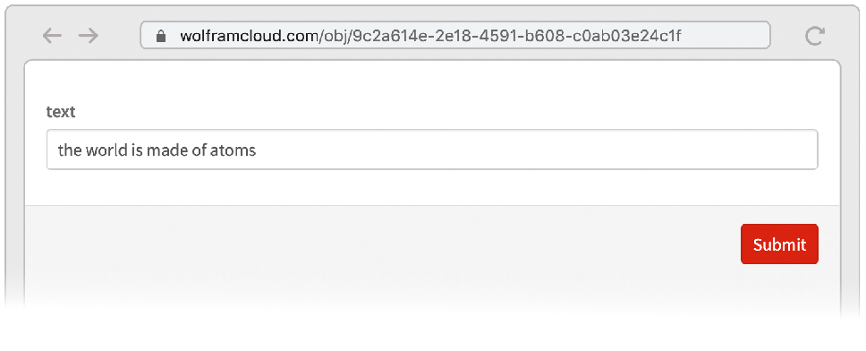
An alternative way to put a model into production is to deploy it on a server or a cloud service. We can, for example, deploy this classifier as a web application. Let’s create a form function, which is a user interface, to interact with the classifier:
Let’s now deploy this form to a cloud service:
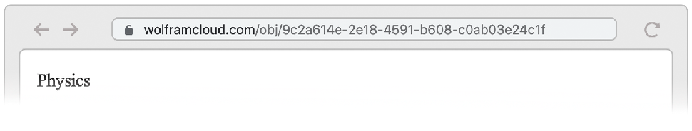
The form is deployed and we can go to the given URL to use it:
Clicking Submit returns physics, as expected:
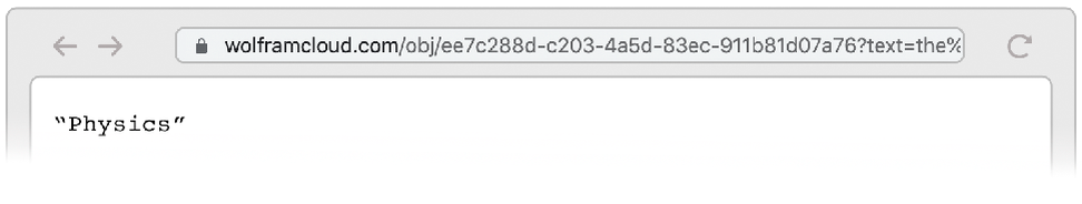
A similar way to deploy a machine learning model is to create an API (application programming interface) so that we can programmatically interact with the classifier as opposed to using a graphical interface. The process is the same as before. We first create an API function:
Then we deploy this API function to a cloud service:
The deployed API function can now be used on our sentence from a web browser by appending the sentence to the given URL:
Creating such an API is probably the most common way to put machine learning models into production.
Once the model is in production, the next step is, of course, to use it but also to monitor its use. Indeed, it is common that a model ends up not being used as intended. For example, some texts given to the classifier might be multi-topic, which violates our assumption, or some of these texts might not even be in English. The goal of this monitoring is to prevent misuse and to improve the model by re-training on data that is more similar to the usage data.
Image Identification
Let’s now come back to the image identification problem presented in the introduction. We are going to improve our mushroom classifier by adding more examples and classes and training a classifier directly with a neural network instead of using an automatic function.
An easy way to get labeled images is from web queries. Let’s load 50 images for each class and label them:
Here are five samples from this dataset:
Let’s now separate this dataset into a training set of 100 examples, a validation set of 50 example, and a test set of 50 examples:
Like a test set, a validation set is a dataset used to measure the performance of a classifier. However, a validation set is generally used during the modeling process, for example, to compare candidate models (see Chapter 5, How It Works), while a test set is only used at the very end of the modeling procedure to obtain an unbiased estimation of the performance of the model.
We now need to define a neural network. Creating good networks from scratch is pretty difficult, so we will use a network that already exists and is suited to classifying images:
Since this network can already recognize images (but not our specific mushrooms), we can also transfer some of its knowledge to our new model. Such a transfer learning procedure is necessary because our dataset is very small (see the Transfer Learning section in Chapter 2, Machine Learning Paradigms).
Okay, let’s first adapt this network to our problem. This network has many layers. Here are the last ones:
We need to replace the last linear layer (![]() ) because it outputs 1000 values while we only want it to return four values (one for each class). Also, we need to replace the post-processor that transforms class probabilities into classes. Here is the modified network:
) because it outputs 1000 values while we only want it to return four values (one for each class). Also, we need to replace the post-processor that transforms class probabilities into classes. Here is the modified network:
And here is the final part of this modified network; note that the last linear layer (![]() ) is not trained yet, hence its color:
) is not trained yet, hence its color:
We can now train this network. Because we do not want to lose knowledge contained in the original network, we only train the last linear layer. All other layers are said to be frozen, and they will not be modified during the training. This is done by setting a learning rate of 0 for these other layers (see Chapter 11, Deep Learning Methods, to understand what a learning rate is):
On the bottom of the result panel, we can see some learning curves that show the cost value (called loss here) during the training procedure. The cost is the objective that we want to minimize (see Chapter 5, How It Works). Note that these learning curves are a bit different from the learning curve seen in the Titanic survival example. The curve that we are really interested in is the blue one because it shows the performance on the validation data (data not seen by the network). We can see that the blue curve is going down, which is what we want, and the curve is still going down at the end of the training, so we would gain by training the network longer.
Although the network is not completely trained, let’s test it. Here is the trained network:
Let’s first try it on some examples that were not in the training set or in the validation set:
Every mushroom is correctly recognized. So far so good. Let’s now do a more thorough analysis by testing all of the examples in the test set:
We can see that the accuracy is around 96%, which is not perfect but much better than the 34% accuracy of the baseline (always predicting the most common class of the test set). On the bottom of the panel, we can see a confusion matrix, which shows the number of test examples of a given class that are classified as another class. We can see that one chanterelle has been classified as a bolete. Let’s extract this example:
This example shows a chanterelle indeed, although it only shows the bottom of the mushroom. In this case, there is nothing wrong with this test example; our model is just not good enough (unless we know that the classifier will always be shown entire mushrooms). In some cases, analyzing classification errors leads to the discovery of wrongly labeled data that should be removed. Such problems in the data can be frequent, which is why it is important to analyze the data in various ways to make sure everything is as we expect, especially for the test set. However, it is also important to keep diversity in the data. We should not confuse removing obvious data errors with removing noisy or weird examples that are very important for creating robust models.
Let’s now extract the three worst classified examples, which means examples for which the probability assigned to the correct class is the lowest:
Such analysis can be instructive for understanding the knowledge gaps of the model. For example, we see that morels in a dish are not well classified. Maybe we should find images of other mushrooms in dishes. Similarly, we could add more images of black boletes or other weird-looking mushrooms. Such data curation is a bit of an art but can be quite effective.
Another way to improve the performance is, of course, to create a substantially larger training set (at least 10 times more examples, such as going from 100 to 1000 or 10000 images). If extra data is not available, we can add synthetic examples by transforming the training images. Typical transformations include blurring, deforming, changing the colors, and so on. This is a classic procedure that is called data augmentation and allows for the injection of knowledge that we have about the data.
To train this network, we froze all layers except the last linear layer. This is good when the number of training examples is small to avoid forgetting the intermediary concepts learned by the original network. Nevertheless, if the number of training data examples is larger, it might be better to unfreeze additional layers, potentially with a lower learning rate (which can depend on their depth in the network).
Yet another way to improve the performance would be to change the pre-trained network, such as by using a better (but bigger in this case) image classifier:
A good pre-trained network is essential when dealing with classic high-dimensional data such as images, audio, or text.
Classification Measures
Measuring the quality of a model is crucial. This can be done using various metrics or measures, and we have encountered some of them previously. These measures can be used to compare models, to figure out if a model should be used or not, or to get insights about how to improve a model. Also, these measures are essential for the learning process itself (see Chapter 5, How It Works). Let’s present the main classification measures.
Decision-Based Measures
The most classic measure is the accuracy, which is simply the fraction of test examples correctly classified. If we predict {"A", "A", "A", "B", B"} when the true classes are {"A", "A", "B", "B", "B"}, the accuracy would be 0.8:
Similarly, the error is the proportion of test examples misclassified:
Note that we used the function MeanAround instead of Mean to obtain uncertainties (±0.2 here). Such statistical uncertainty is due to the finite number of test examples, and the simplest way to reduce it is to add more test examples. A useful fact to remember is that this uncertainty behaves like the inverse of a square root with the number of test examples. This means that we would need to multiply the number of test examples by 4 in order to halve the uncertainty.
Accuracy and error are popular measures for classifiers because they are easy to compute and to understand. Nevertheless, these measures can be misleading. For example, I can predict with an accuracy higher than 99.99% that you are not experiencing a solar eclipse right now. This does not mean that I have superpowers but only that eclipses are very rare. So is our 80% accuracy a good result? This depends on the application, of course, but we should at least compare this measure with a baseline. The simplest baseline is to always predict the most common class, which is "B" here:
Another comparison point would be the accuracy of the best performing system currently available for this task.
Let’s now measure things in more detail and look at the fraction of class "A" examples that are correctly classified, and similarly for class "B":
This sort of per-class accuracy is called the recall. We could also look at the fraction of correct classification amongst all examples that are classified as "A", and similarly for class "B":
This sort of accuracy from the point of view of the predicted classes is called the precision. The precision tells us how much to trust a given prediction. Here, we would trust the prediction "B" (if it was not for statistical uncertainties). Depending on the task, one might want to optimize for a better recall or for better precision. For example, in a medical test, we might care more about not missing a disease than wrongly classifying a healthy patient. Precision and recall are often used to assess the performance of binary classifiers. Generally, the values are only reported for one of the two classes, which is then called the positive class (the other class is called the negative class). In our medical test, the positive class would certainly be the “diseased” class.
There are also measures that combine the precision and recall, such as the F1 score:
The F1 score is the harmonic mean of the precision and recall, which puts a heavy penalty if either the precision or recall is bad. Such measures can be used to understand which classes are performing well and which ones are not.
There are plenty of more advanced measures based on class decisions that try to capture how good the model is. Notable ones are the area under the ROC curve, Matthews correlation coefficient, and Cohen’s kappa, but we won’t present them here.
Measures based on class decisions are generally quite interpretable, which makes them useful for understanding and communicating how good the model is. The issue with decision-based measures is that they don’t take into account the predicted probabilities and, therefore, cannot completely capture the performance of a model.
Confusion Matrix
To understand better the performance of a classifier, we can visualize its confusion matrix computed from a test set:
This matrix shows the number of examples of a given class classified as another class. Here is a larger confusion matrix obtained from a handwritten digit classifier:
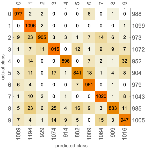
This allows for easy visualization of which class is confused with which other class. The next step would be to look directly at test examples, such as the ones corresponding to a particular confusion.
Likelihood
The measures described so far are purely based on class decisions, but we often care about class probabilities as well. Let’s now introduce the likelihood, which is the main measure computed from class probabilities.
As before, let’s assume that the correct classes are as follows:
Now let’s assume that the classifier returned these class probabilities:
Here are these probabilities with the correct classes highlighted:
The likelihood is simply the product of the probabilities attributed to correct classes:
As usual, we want to compare this result with a baseline, such as the likelihood obtained by probabilities corresponding to the frequencies in the test set:
In this case, the classifier is better than the baseline according to this measure.
If we had more examples, the likelihood would become very small because we are multiplying numbers smaller than 1. To make things more practical, we generally compute the log-likelihood instead, which we can compute by summing the log of the probabilities:
Also, let’s compute an average instead of a sum, just so that the measure does not naturally increase with the number of examples:
Finally, let’s add a minus sign because, by convention, we prefer to have something to minimize rather than to maximize in machine learning (see Chapter 5, How It Works):
This final measure is very common and has many names such as negative log-likelihood (NLL) or mean cross-entropy. Mathematically, we can write it as follows:
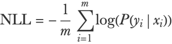
Here xi and yi are the input and the output of example i and m is the number of examples.
One issue with this measure is that it is less interpretable than the accuracy. One way to mitigate this is to compute the geometric mean of the correct-class probabilities instead, which is the same measure but easier to interpret:
Here we would say that the classifier typically assigns a probability of 66% to the correct class, which can be compared to the class-frequency baseline:
The likelihood measure (and its variations) is central to machine learning. It is considered to be the most agnostic way to measure how good a probabilistic classifier is. Most probabilistic models, including classifiers, are trained by optimizing this measure. This does not mean that the likelihood is a perfect measure for every application though. For example, if you only care about class decisions and not class probabilities, the likelihood is probably not the best measure to focus on. There are other standard probabilistic measures (such as the Brier score), but the likelihood is by far the most used.
Probability Calibration
There is one other kind of probabilistic measurement that is worth mentioning and concerns the reliability of the classifier, also known as the probability calibration. Reliability is not really telling us how “good” a model is but rather if we can rely on its probabilities. Let’s look at what this means with an example.
Let’s consider the following training and test set:
The goal here is to learn to recognize handwritten digits. Here are examples from the test set:
Let’s train two classifiers using different methods and without probability recalibration:
Each learned model can give us its belief about the class of a new image in terms of probabilities:
Here the classifier gives about a 71% chance of this image being a 7. Of course, we can see that it is actually a 7, so this probability is completely relative to the understanding of the model and not a “true” probability. The question is, can we rely on these probabilities to make decisions or are they meaningless aside from telling us which class is the most likely? For example, if we were to only trust the model when it predicts a class with a probability higher than 0.9, would more than 90% of the decisions made by the model be correct? This sort of question is answered by doing a reliability analysis of the model.
Let’s display the reliability curves for each classifier. These curves show the frequency of correct outcome for a given predicted probability. They are computed using a histogram on the test set. All the predicted probabilities that fall into a range, such as 0.7<p<0.71, are gathered, and the frequency of their actual realization is computed:
The curve for a perfectly reliable classifier would be on the diagonal. We can see that the first classifier is severely underconfident. For example, when it believes something has a 70% chance of being true, we can expect the actual realization to happen 99% of the time! Inversely, the second classifier is a bit overconfident. To obtain a more reliable classifier, we can calibrate probabilities by training a small model on top of the original model (typically using the log-probabilities as input). The Classify function automatically performs this calibration:
Here probabilities are quite well calibrated; the classifier is reliable. We should remember that reliability is only valid if test examples come from the same distribution as the training examples. If this classifier is used on examples that come from a different distribution, the classifier would not be calibrated (see the iid assumption explained in Chapter 5, How It Works).
Reliability does not say much about how good a model is because even a bad classifier can be calibrated by saying “I don’t know” all the time, but it is helpful to know if we can trust a prediction or not. Reliability is particularly important for sensitive applications, such as disease diagnostics.
From Probabilities to Decisions
As we saw earlier, most classifiers return class probabilities that correspond to their belief about the class of a given example. There is more information in such probabilities than in a pure class prediction. Let’s look at how we can use this to our advantage.
Let’s imagine that we used one of our mushroom classifiers during a walk in a forest to identify this mushroom (which no one should do given how crude this classifier is!):

Let’s now imagine that the classifier returned the following probabilities:
This means that given the examples that the classifier saw during its training and given what it “understood” about them, there is a 90% chance of this mushroom being a morel. Can we use these probabilities? There are several things to take into account to figure this out.
First, these probabilities are made under the assumption that the new image comes from the same distribution as the training images. This is related to the iid assumption, which is explained in Chapter 5. More simply put, this image should have been generated from the same process as the training images. For example, if the training images are pictures made by a particular camera, then the new image should also be a picture made by this specific camera. In practice, it is pretty hard to have this assumption completely satisfied, but we can get close by diversifying the training data as much as possible.
Okay, so let’s assume that the new image comes from the same distribution as the training images. The next step is to make sure that the probabilities are calibrated (see the previous section). As it happens, modern neural networks tend to be overconfident, so this calibration step is important if we want to use these probabilities and not just the predictions.
The next thing to consider is the prior distribution of classes (a.k.a. class priors) for our new image. For example, let’s assume that there are as many boletes as morels and as chanterelles in our forest at this time of the year. Since our classifier has been trained with a balanced training set, we don’t have to do anything and can keep class probabilities as they are. However, let’s say that we know that in this specific forest, there is a 70% chance of encountering a morel, a 20% chance for a chanterelle, and only a 10% chance for a bolete. Our class prior is then:
This is different from the training prior:
We should take into account this new prior and update the class probabilities. This update is done by multiplying the probabilities with the new prior, dividing by the old one, and then normalizing everything so that the probabilities sum to 1, which is a Bayesian update (see Chapter 12, Bayesian Inference):
We see that the probability of a morel went from 90% to about 97.8% when taking into account our class prior.
Okay, so now that we are done with these steps, we can start using these probabilities. Should we label our mushroom as a morel? Well, identifying a mushroom has consequences since we might eat it and get poisoned if we are wrong. One simple strategy to make a decision here is to set a probability threshold under which we do not trust the classifier and bring the mushroom to an expert instead (or not pick the mushroom at all). For example, if we had set a probability threshold of 99%, this particular classification would be rejected. The value for this rejection threshold is entirely application dependent, which, in this case, depends on how much risk we are willing to take. Such thresholding is used a lot in practice for its simplicity.
Another—albeit more cumbersome—strategy to obtain a label given probabilities is to use decision theory. Decision theory is a formal way of making decisions under uncertainty. The basic idea is to set up a utility function that captures our “happiness” about a decision given the true class: f(true class,decision)->utility. Here the utility function needs to be defined for every possible actual class and decision. We can thus represent it with a utility matrix. The standard utility matrix is the identity:
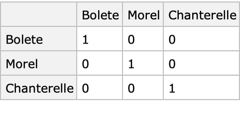
The decision is made by maximizing the expected utility given our belief. For example, let’s extract the utility vector corresponding to the "Bolete" decision:
We can compute the expected utility of the "Bolete" decision from this vector and the class probabilities:
Then we could do this for other possible classes and pick the one that maximizes the expected utility. In this case, the expected utilities are equal to the probabilities because we used an identity matrix. This means that, by default, the best decision is the class that has the highest probability, which is not surprising.
Now let’s change our utility matrix. For example, we might know that there are dangerous boletes in this forest that we should not eat, but that morels and chanterelles are fine. We thus really do not want to misclassify a bolete as something else. Let’s encode this in a new utility:
We can see that our utility is now -200 when we decide that it is a morel or a chanterelle when it was in fact a bolete. Let’s compute the expected utility for every possible decision:
We can see that the highest expected utility is now for the decision "Bolete" even though the probability of bolete was low because it is the safe decision to make. We could also include alternative decisions such as "ask an expert".
Here is an example of such a utility:
And here are the corresponding expected utilities:
We would thus ask an expert in this case.
Using decision theory is useful for sensitive applications, such as medical testing, but also for applications where outcomes are clearly quantified (e.g. when trading or betting). The drawbacks are that decision theory is harder to use than a simple thresholding and, importantly, that it is often difficult to transcribe our fuzzy goals into a utility function (it can be a useful exercise though). Nevertheless, decision theory constitutes the proper way to take decisions under uncertainty and would certainly gain to be used more.
| ■ | Classification is the task of learning to predict to which class a new example belongs. |
| ■ | Examples to be classified can be pieces of text, images, or structured data amongst other things. |
| ■ | Classifiers can generally return class probabilities. |
| ■ | A classifier must be tested on data that has not been used for training purposes. |
| ■ | Accuracy and likelihood are the two main classification measures. |
| ■ | Diversifying the origin of the data, adding more examples, and adding/extracting better features are generally the ways to improve a classifier. |
| ■ | Exploratory data analysis is an important first step for a machine learning project. |
| numeric variable | variable whose values are numbers or numeric quantities | |
| categorical variable nominal variable | variable whose values are categories/classes | |
| feature type | the variable type to which a feature belongs (numeric, categorical, text, etc.) | |
| class | named label such as "dog", "cat", or "tree", also called a categorical value or a nominal value | |
| classification | task of predicting a categorical variable | |
| binary classification | classification task that has only two possible classes | |
| multiclass classification | classification task that has more than two classes | |
| classifier | machine learning model able to classify new examples | |
| class probabilities | probabilities returned by a classifier for a given input | |
| probabilistic model | model that can provide class probabilities or a predictive distribution | |
| decision boundary | region where the classification changes from one class to another | |
| multi-label classification | classification task for which each example can have more than one class | |
| serialization | process of converting a model into a format that can be stored (e.g. in a file) to be reconstructed later | |
| exploratory data analysis | initial analysis of a dataset using statistical metrics or data visualization methods, the goal is to understand what the dataset is to figure out what to do with it | |
| feature importance importance value | value that indicates the importance of a given feature in a model for a specific prediction or for a set of predictions | |
| SHAP | classic method to estimate the importance of each feature for a given prediction | |
| odds | measure of the likelihood of a particular event, the odds of an event where probability p is | |
| balanced dataset | dataset containing about the same number of examples for all possible classes | |
| imbalanced dataset | dataset containing substantially more examples for some classes than for other classes | |
| data augmentation | adding synthetic training examples created from existing ones to obtain a larger dataset, typically used to augment the number of images by rotating them, blurring them, etc. | |
| training set | dataset used to learn a model | |
| validation set | dataset used to measure the performance of a model during the modeling process (for example, to compare candidate models) | |
| test set | dataset used to measure the performance of a model after the modeling process to obtain an unbiased estimation of the performance |
| measure metric | computed quantity that informs about the performance of a model, such as the accuracy; measures are typically computed on a validation or a test set | |
| cost functioncost value | objective that we want to minimize during the learning process | |
| learning curve | curve showing the performance of a machine learning model as function of a parameter of interest, such as the number of training examples or the training time | |
| accuracy | proportion of examples that are correctly classified in a given dataset | |
| error | proportion of examples that are incorrectly classified in a given dataset | |
| recall | proportion of examples that are correctly classified amongst examples of a given class | |
| precision | proportion of examples that are correctly classified amongst examples that are classified as a given class | |
| positive class | in binary classification problems, the special class for which binary decision measures (recall, precision, etc.) are reported | |
| confusion matrix | matrix containing, for every possible class pair, the number of test examples belonging to a class that are classified as another class | |
| likelihood | product of the probabilities attributed to correct classes | |
| log-likelihood | log of the likelihood | |
| negative log-likelihood mean cross-entropy | opposite of the log-likelihood per number of examples | |
| reliability calibration probability calibration | ability for a model to correctly assess its own uncertainty | |
| calibrating a model | correcting a model for it to become reliable | |
| reliability curve | curve showing the actual frequency of an outcome when predicting this outcome with a given probability | |
| underconfident model | model whose predicted uncertainty is typically larger than it should be given its predictions | |
| overconfident model | model whose predicted uncertainty is typically smaller than it should be given its predictions |
| prior distribution class priors | model assumption about class frequencies | |
| rejection threshold | probability threshold under which we reject the decision of a classifier | |
| decision theory | procedure to make decisions under uncertainty | |
| utility function | function that captures our “happiness” about a decision given the true class | |
| utility matrix | matrix representing the utility for every possible decision and true class | |
| expected utility | average utility of a decision according to some beliefs |