ボックス内の量子力学的粒子を観察する: Wolfram言語 11の新機能

ボックス内の量子力学的粒子を観察する

2辺の長さがとである長方形内を自由に運動する粒子は，二次元の時間依存のシュレディンガー方程式と，境界上で波動関数がゼロであるという境界条件によって記述される．

In[1]:=

eqn = I D[\[Psi][x, y, t], t] == -\[HBar]^2/(2 m)
     Laplacian[\[Psi][x, y, t], {x, y}];

In[2]:=

bcs = {\[Psi][0, y, t] == 0, \[Psi][xMax, y, t] == 
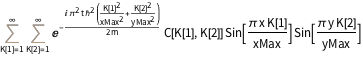
    0, \[Psi][x, yMax, t] == 0, \[Psi][x, 0, t] == 0};

この方程式は，いわゆる固有状態の形式的な無限和で表される一般解を持つ．

In[3]:=

DSolveValue[{eqn, bcs}, \[Psi][x, y, t], {x, y, t}]

Out[3]=

規格化された固有状態に等しい初期条件を定義する．

In[4]:=

initEigen = \[Psi][x, y, 0] == 
   2 /Sqrt[xMax yMax] Sin[(\[Pi] x)/xMax] Sin[(\[Pi] y)/yMax];

この場合，解は，初期条件に，時間に依存する絶対値1の係数を乗じただけのものになる．

In[5]:=

DSolveValue[{eqn, bcs, initEigen}, \[Psi][x, y, t], {x, y, t}]

Out[5]=

固有状態の和である初期条件を定義する．初期条件は固有状態ではないので，粒子の位置についての確率密度は時間依存となる．

In[6]:=

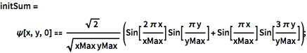
initSum = \[Psi][x, y, 0] == 
   Sqrt[2]/Sqrt[
    xMax yMax] (Sin[(2 \[Pi] x)/xMax] Sin[(\[Pi] y)/yMax] + 
      Sin[(\[Pi] x)/xMax] Sin[(3 \[Pi] y)/yMax]);

新しい初期条件で解く．

In[7]:=

sol = DSolveValue[{eqn, bcs, initSum}, \[Psi][x, y, t], {x, y, t}]

Out[7]=

換算プランク(Planck)定数，電子の質量，原子サイズのボックスの値を，電子の質量，ナノメートル，フェムト秒の単位を使って代入し，確率密度を計算する．

In[8]:=

\[HBar] = 
 QuantityMagnitude[Quantity[1., "ReducedPlanckConstant"], 
  "ElectronMass" * ("Nanometers")^2/"Femtoseconds"]

Out[8]=

In[9]:=

\[Rho][x_, y_, t_] = 
 FullSimplify[ComplexExpand[Conjugate[sol] sol]] /. {m -> 1, 
   xMax -> 1, yMax -> 1}

Out[9]=

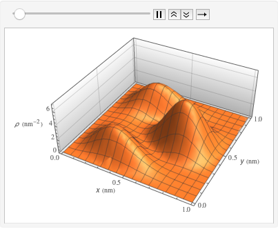
ボックス内の確率密度を時間の経過とともに可視化する．

In[10]:=

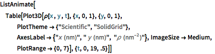
ListAnimate[
 Table[Plot3D[\[Rho][x , y , t], {x, 0, 1}, {y, 0, 1}, 
   PlotTheme -> {"Scientific", "SolidGrid"}, AxesLabel -> {"\!\(\*
StyleBox[\"x\", \"SO\"]\) (nm)", " \!\(\*
StyleBox[\"y\", \"SO\"]\) (nm)", "\!\(\*
StyleBox[\"\[Rho]\", \"SO\"]\) (\!\(\*SuperscriptBox[\(nm\), \
\(-2\)]\))"}, ImageSize -> Medium, PlotRange -> {0, 7}], {t, 0, 
   19, .5}]]