High-Performance Numeric Solution of Polynomial Systems
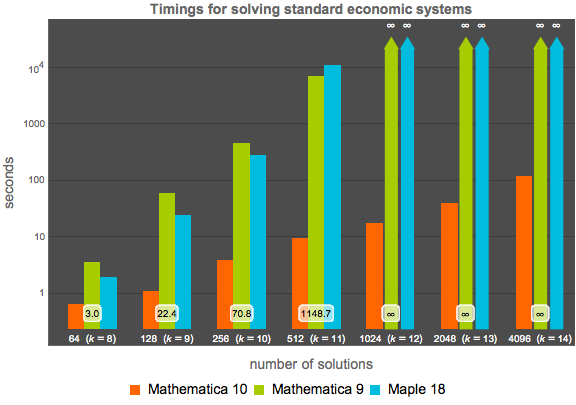
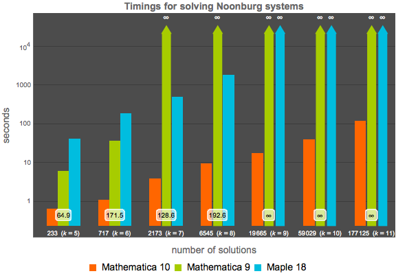
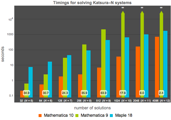
Mathematica 10 includes a new homotopy-based numerical polynomial solver. This method is automatically selected when appropriate. The following charts compare the timing of this new algorithm with Mathematica 9's Gröbner-basis method and the faster of Maple 18's solve or Homotopy commands. All tests were performed on a 16-core, 2.40 GHz 64-bit Linux system with Hyper-Threading enabled and a time limit of 12 hours.
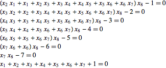
Comparison for a standard economics system in  variables, total degree
  , and
, and  distinct solutions, given by the following formula.
| In[1]:= | X |
For example, for  the system takes the following form.
| In[2]:= | X |
| Out[2]//TraditionalForm= | |
 | |
 |
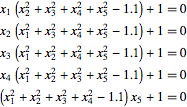
Comparison for the standard Noonburg neural-network system, given by the following formula. For  variables, this system has total degree
  and
and  different solutions.
| In[3]:= | X |
For example, in five variables the system takes the following form.
| In[4]:= | X |
| Out[4]//TraditionalForm= | |
 | |
 |
Comparison for the standard Katsura- system of ferromagnetic lattice probabilities, which in
  variables has total degree
  and
and  different solutions. The order-
 system takes the following form.
| In[5]:= | 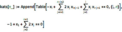 X |
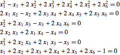
For example, for  the system has six equations in six unknowns.
| In[6]:= | X |
| Out[6]//TraditionalForm= | |
 | |
 |