Eigenvalue Spacings of Gaussian Distributions

The eigenvalue spacings (differences of consecutive eigenvalues) of matrix distributions have a universal limiting form that is observed in many systems in nature, such as the energy-level spacings of heavy atoms.

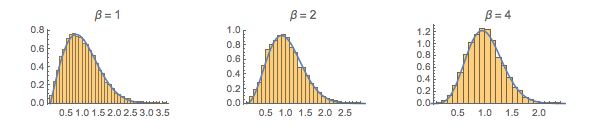
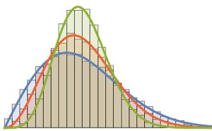
Sample eigenvalue spacing of 2×2 matrices from different Gaussian ensembles.

In[1]:=

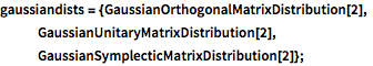
gaussiandists = {GaussianOrthogonalMatrixDistribution[2], GaussianUnitaryMatrixDistribution[2], GaussianSymplecticMatrixDistribution[2]};

In[2]:=

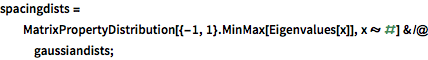
spacingdists = MatrixPropertyDistribution[{-1, 1}.MinMax[Eigenvalues[x]], x \[Distributed] #] & /@ gaussiandists;

In[3]:=

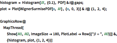
gaps = Normalize[RandomVariate[#, 10000], Mean] & /@ spacingdists;

Compare the histograms for each distribution with their closed form, also known as Wigner surmise for Dyson indices of , , and .

In[4]:=

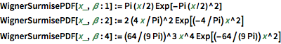
WignerSurmisePDF[x_, \[Beta] : 1] := Pi (x/2) Exp[-Pi (x/2)^2] WignerSurmisePDF[x_, \[Beta] : 2] := 2 (4 x/Pi)^2 Exp[(-4/Pi) x^2] WignerSurmisePDF[ x_, \[Beta] : 4] := (64/(9 Pi))^3 x^4 Exp[(-64/(9 Pi)) x^2]

In[5]:=

histogram = Histogram[#, {0.1}, PDF] & /@ gaps; plot = Plot[WignerSurmisePDF[x, #] , {x, 0, 3}] & /@ {1, 2, 4}; GraphicsRow@ MapThread[ Show[#1, #2, ImageSize -> 180, PlotLabel -> Row[{"\[Beta] = ", #3}]] &, {histogram, plot, {1, 2, 4}}]

Out[5]=