Matrix Normal and Matrix T Distributions

Matrix normal and matrix distributions are matrix variate normal and distributions with specified row and column scale matrices. Typical uses include time series analysis, random processes, and multivariate regression.

Given the scale matrices Σ_row and Σ_col, matrix normal distribution has probability density proportional to . Sample from a matrix normal distribution.

In[1]:=

Subscript[\[CapitalSigma], row] = {{1, 0.9}, {0.9, 1}}; Subscript[\[CapitalSigma], col] = {{1, -0.9}, {-0.9, 1}};

In[2]:=

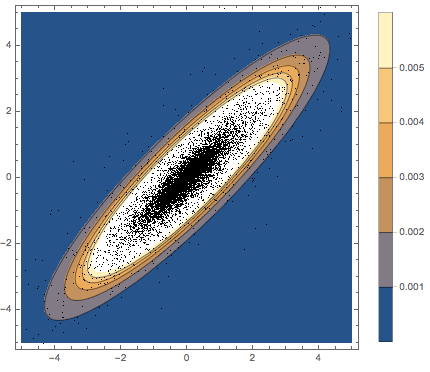
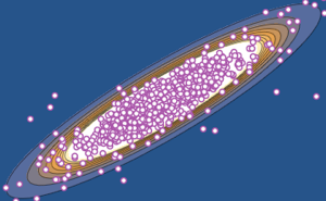
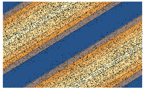
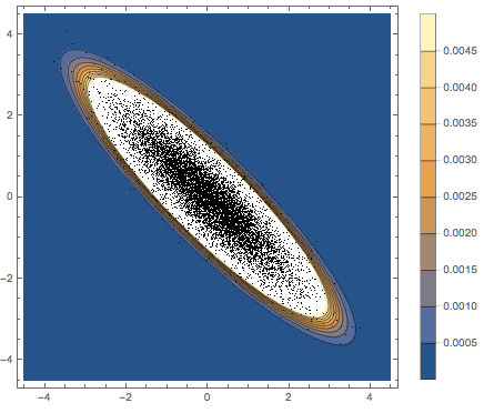
RandomVariate[ MatrixNormalDistribution[Subscript[\[CapitalSigma], row], Subscript[\[CapitalSigma], col]]]

Out[2]=

Visualize the sampled row vectors on a scatter plot and compare it with the density function.

In[3]:=

sample = RandomVariate[ MatrixNormalDistribution[Subscript[\[CapitalSigma], row], Subscript[\[CapitalSigma], col]], 10^4]; firstrows = sample[[All, 1]];

In[4]:=

Show[ContourPlot[ PDF[MultinormalDistribution[{0, 0}, Subscript[\[CapitalSigma], col] ], {x, y}], {x, -4.5, 4.5}, {y, -4.5, 4.5}, PlotPoints -> 30, PlotTheme -> "Detailed", ImageSize -> Medium], ListPlot[firstrows, ImageSize -> Medium, PlotTheme -> "Detailed", PlotStyle -> Black]]

Out[4]=

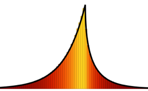
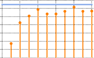
Visualize the sampled column vectors on a histogram and compare it with the density function.

In[5]:=

firstcols = sample[[All, All, 1]];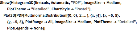

In[6]:=

Show[Histogram3D[firstcols, Automatic, "PDF", ImageSize -> Medium, PlotTheme -> "Detailed", ChartStyle -> "Pastel"], Plot3D[PDF[ MultinormalDistribution[{0, 0}, Subscript[\[CapitalSigma], row] ], {x, y}], {x, -5, 5}, {y, -5, 5}, PlotRange -> All, ImageSize -> Medium, PlotTheme -> "Detailed", PlotLegends -> None]]

Out[6]=

Similar to Student and multivariate distributions, matrix distribution is a mixture of matrix normal distribution with inverse Wishart distributed scale parameter. Sample from a matrix distribution.

In[7]:=

RandomVariate[ MatrixTDistribution[Subscript[\[CapitalSigma], row], Subscript[\[CapitalSigma], col], 3]]

Out[7]=

Generate a set of matrix distributed matrices.

In[8]:=

sample = RandomVariate[ MatrixTDistribution[Subscript[\[CapitalSigma], row], Subscript[\[CapitalSigma], col], 3], 10^4];

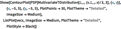
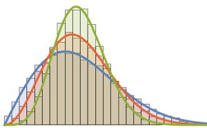
Lower-dimensional projections of matrix distributed variates are Student and multivariate distributed. Project the sample to two-dimensional vectors and verify the goodness of fit.

In[9]:=

v = {1, 2}; vecs = sample.v;

In[10]:=

DistributionFitTest[vecs, MultivariateTDistribution[ Subscript[\[CapitalSigma], row] (v.Subscript[\[CapitalSigma], col].v)/3, 3]]

Out[10]=

Visualize the projected data on a scatter plot and compare it with the density function.

In[11]:=

Show[ContourPlot[ PDF[MultivariateTDistribution[ Subscript[\[CapitalSigma], row] (v.Subscript[\[CapitalSigma], col].v)/3, 3], {x, y}], {x, -5, 5}, {y, -5, 5}, PlotPoints -> 30, PlotTheme -> "Detailed", ImageSize -> Medium], ListPlot[vecs, ImageSize -> Medium, PlotTheme -> "Detailed", PlotStyle -> Black]]

Out[11]=