Solve the Wave Equation Using Its Fundamental Solution
Define a wave operator in one spatial dimension.
In[1]:=
waveOperator = \!\(
\*SubscriptBox[\(\[PartialD]\), \({t, 2}\)]\(u[x, t]\)\) - \!\(
\*SubscriptBox[\(\[PartialD]\), \({x, 2}\)]\(u[x, t]\)\);
Obtain its fundamental solution using GreenFunction.
In[2]:=
gf[x_, t_, y_, s_] =
 GreenFunction[waveOperator, u[x, t], {x, -\[Infinity], \[Infinity]},
  t, {y, s}]
Out[2]=
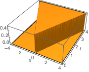
Plot the fundamental solution.
In[3]:=
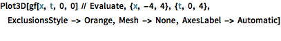
Plot3D[gf[x, t, 0, 0] // Evaluate, {x, -4, 4}, {t, 0, 4},
 ExclusionsStyle -> Orange, Mesh -> None, AxesLabel -> Automatic]
Out[3]=
Define a forcing function.
In[4]:=
f[y_, s_] := Cos[y] E^(-s)Solve the wave equation with this forcing term by evaluating the convolution integral  .
.
In[5]:=
sol = Integrate[
   gf[x, t, y, s] f[y, s], {y, -\[Infinity], \[Infinity]}, {s,
    0, \[Infinity]}, Assumptions -> t > 0 && Im[x] == 0] //
  FullSimplify
Out[5]=
Obtain the result using DSolveValue with homogeneous initial conditions.
In[6]:=
initialc = {u[x, 0] == 0, Derivative[0, 1][u][x, 0] == 0};In[7]:=
DSolveValue[{waveOperator == f[x, t], initialc}, u[x, t], {x, t}]Out[7]=
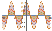
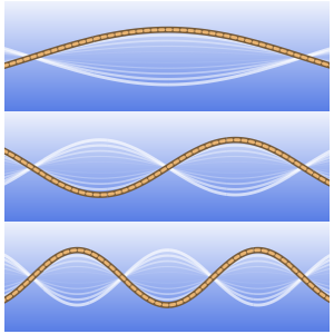
Visualize the standing wave generated by the solution.
In[8]:=
Plot[Table[sol, {t, 0, 1, 0.2}] // Evaluate, {x, -10, 10},
 Filling -> Axis]
Out[8]=