Solve a Boundary Value Problem Using a Green's Function

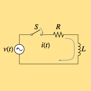
Solve the following second-order differential equation subject to the given homogeneous boundary conditions.

In[1]:=

eqn = -u''[x] - u'[x] + 6 u[x] == f[x];

In[2]:=

bc0 = u[0] == 0;

In[3]:=

bc1 = u[1] == 0;

The forcing term is given by the following function f[x].

In[4]:=

f[x_] := E^(-a x)

Compute the Green's function for the corresponding differential operator.

In[5]:=

gf[y_, x_] = GreenFunction[{eqn[[1]], bc0, bc1}, u[x], {x, 0, 1}, y]

Out[5]=

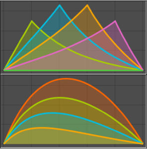
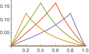
Plot the Green's function for different values of lying between 0 and 1.

In[6]:=

Plot[Table[gf[y, x], {y, 0, 1, 0.2}] // Evaluate, {x, 0, 1}]

Out[6]=

The solution of the original differential equation with the given forcing term can now be computed using a convolution integral on the interval .

In[7]:=

sol = Integrate[gf[y, x] f[y], {y, 0, 1}, Assumptions -> 0 < x < 1] // Simplify

Out[7]=

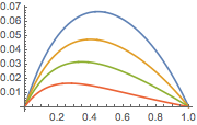
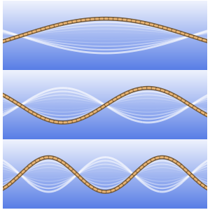
Plot the solution for different values of the parameter .

In[8]:=

Plot[Table[sol, {a, {1/4, 1, 2, 4}}] // Evaluate, {x, 0, 1}]

Out[8]=