| 21 | Graphs and Networks |
A graph is a way of showing connections between things—say, how webpages are linked, or how people form a social network.
Let’s start with a very simple graph, in which 1 connects to 2, 2 to 3 and 3 to 4. Each of the connections is represented by (typed as ->).
A very simple graph of connections:
In[1]:=
Out[1]=
Automatically label all the “vertices”:
In[2]:=
Out[2]=
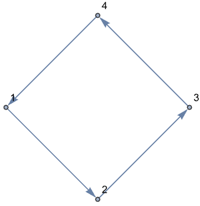
Let’s add one more connection: to connect 4 to 1. Now we have a loop.
Add another connection, forming a loop:
In[3]:=
Out[3]=
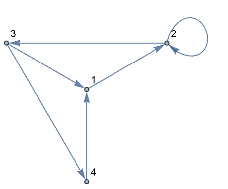
Add two more connections, including one connecting 2 right back to 2:
In[4]:=
Out[4]=
As we add connections, the Wolfram Language chooses to place the vertices or nodes of the graph differently. All that really matters for the meaning, however, is how the vertices are connected. And if you don’t specify otherwise, the Wolfram Language will try to lay the graph out so it’s as untangled and easy to understand as possible.
There are options, though, to specify other layouts. Here’s an example. It’s the same graph as before, with the same connections, but the vertices are laid out differently.
A different layout of the same graph (check by tracing the connections):
In[5]:=
Out[5]=
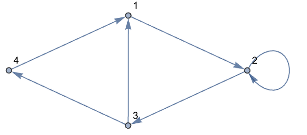
You can do computations on the graph, say finding the shortest path that gets from 4 to 2, always following the arrows.
The shortest path from 4 to 2 on the graph goes through 1:
In[6]:=
Out[6]=
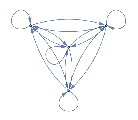
Now let’s make another graph. This time let’s have 3 nodes, and let’s have a connection between every one of them.
Start by making an array of all possible connections between 3 objects:
In[7]:=
Out[7]=
The result here is a list of lists. But what Graph needs is just a single list of connections. We can get that by using Flatten to “flatten” out the sublists.
Flatten “flattens out” all sublists, wherever they appear:
In[8]:=
Out[8]=
Get a “flattened” list of connections from the array:
In[9]:=
Out[9]=
In[10]:=
Out[10]=
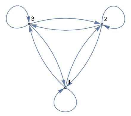
Generate the completely connected graph with 6 nodes:
In[11]:=
Out[11]=
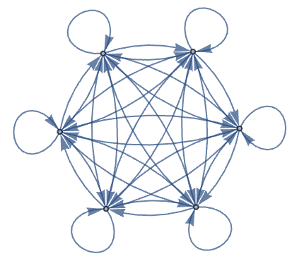
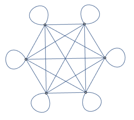
Sometimes the “direction” of a connection doesn’t matter, so we can drop the arrows.
The “undirected” version of the graph:
In[12]:=
Out[12]=
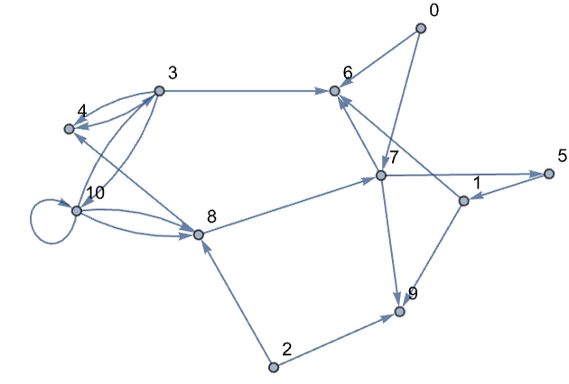
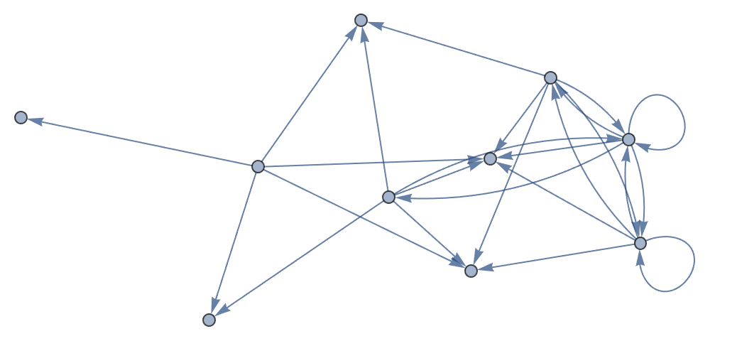
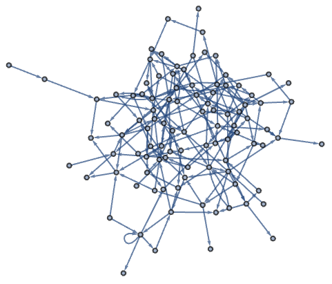
Now let’s make a graph with random connections. Here is an example with 20 connections between randomly chosen nodes.
Make a graph with 20 connections between randomly chosen nodes numbered from 0 to 10:
In[13]:=
Out[13]=
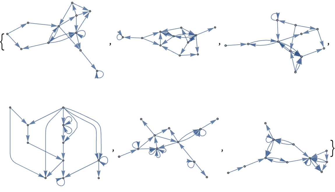
You’ll get a different graph if you generate different random numbers. Here are 6 graphs.
Six randomly generated graphs:
In[14]:=
Out[14]=
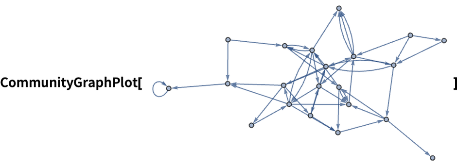
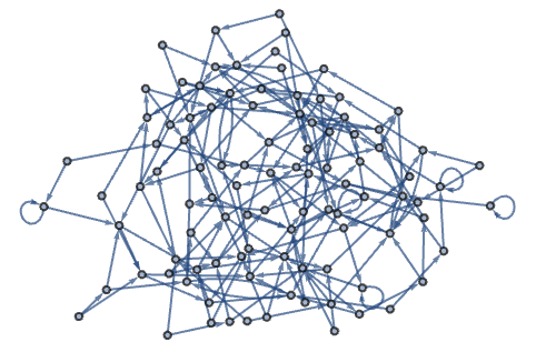
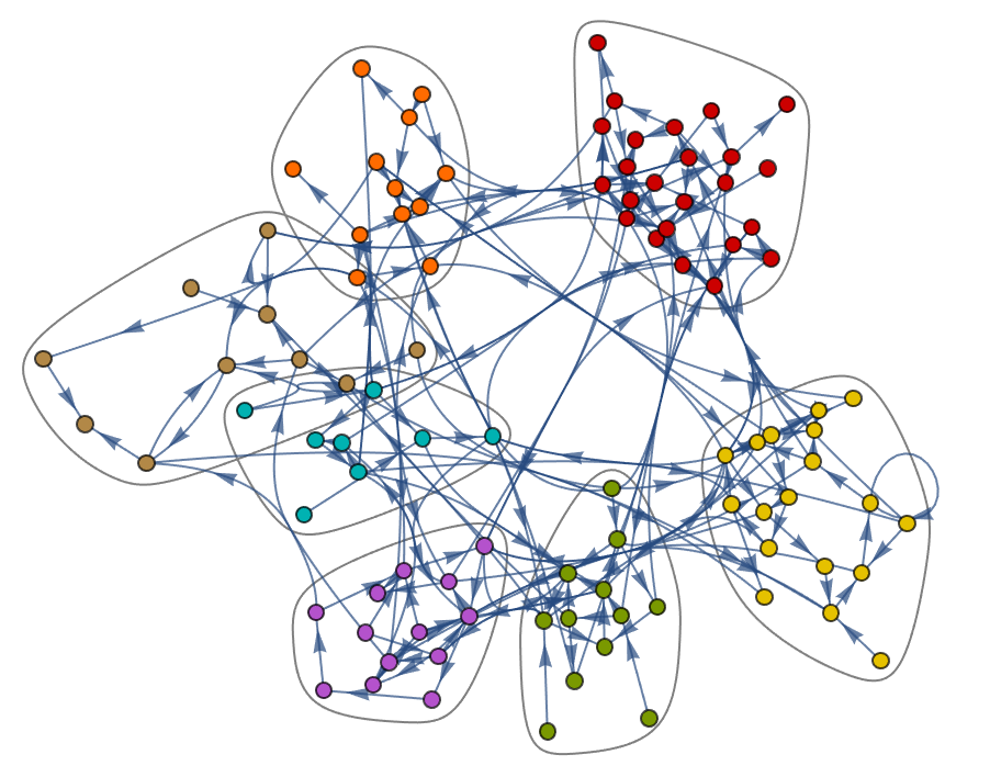
There’s lots of analysis that can be done on graphs. One example is to break a graph into “communities”—clumps of nodes that are more connected to each other than to the rest of the graph. Let’s do that for a random graph.
In[15]:=
Out[15]=
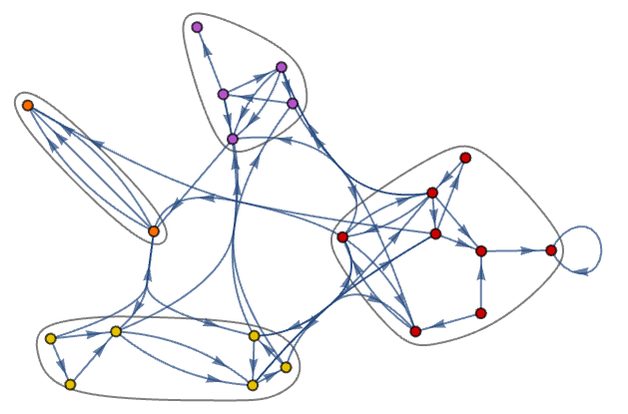
The result is a graph with the exact same connections as the original, but with the nodes arranged to illustrate the “community structure” of the graph.
| Graph[{ij,...}] | a graph or network of connections | |
| UndirectedGraph[{ij, ...}] | a graph with no directions to connections | |
| VertexLabels | an option for what vertex labels to include (e.g. All) | |
| FindShortestPath[graph,a,b] | find the shortest path from one node to another | |
| CommunityGraphPlot[list] | display a graph arranged into “communities” | |
| Flatten[list] | flatten out sublists in a list |
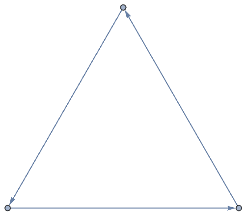
21.1Make a graph consisting of a loop of 3 nodes. »

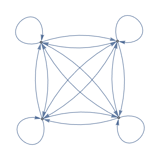
21.2Make a graph with 4 nodes in which every node is connected. »
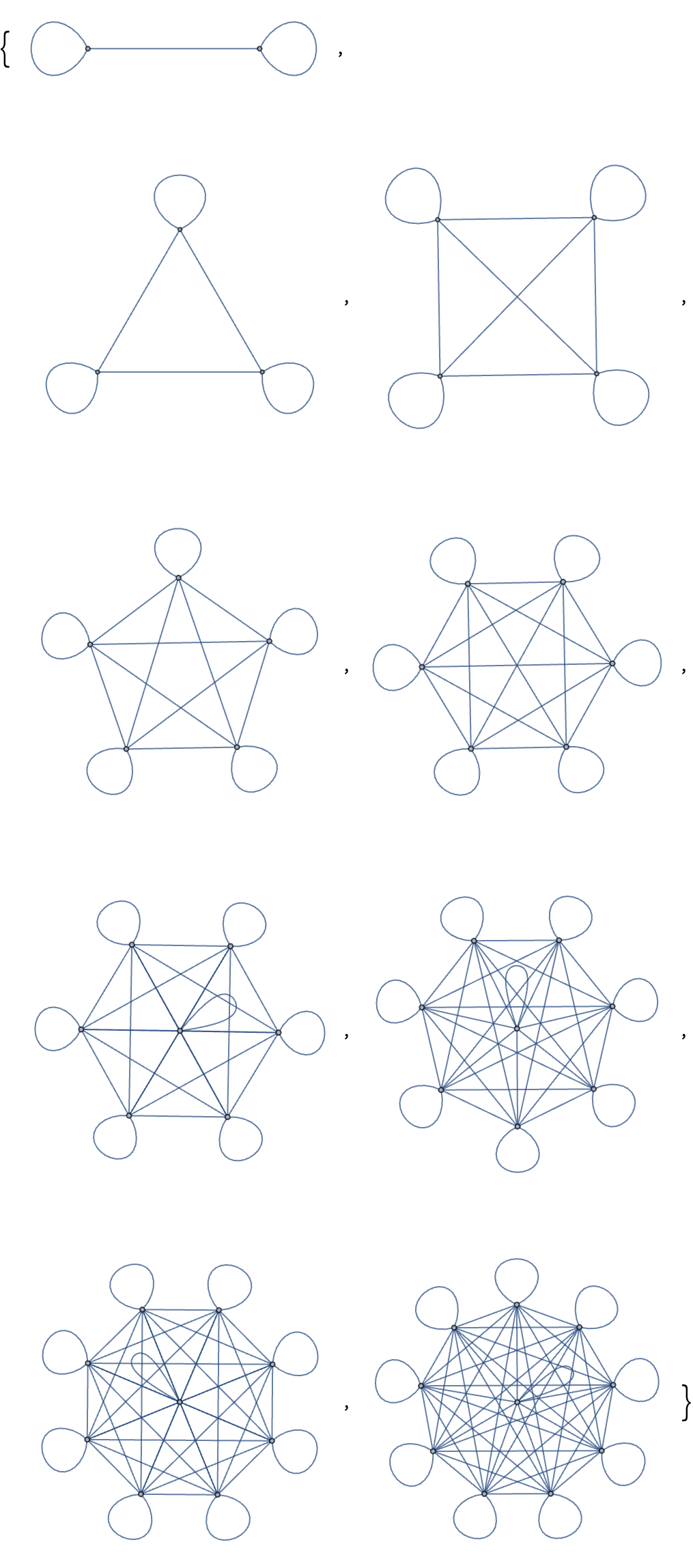
21.3Make a table of undirected graphs with between 2 and 10 nodes in which every node is connected. »
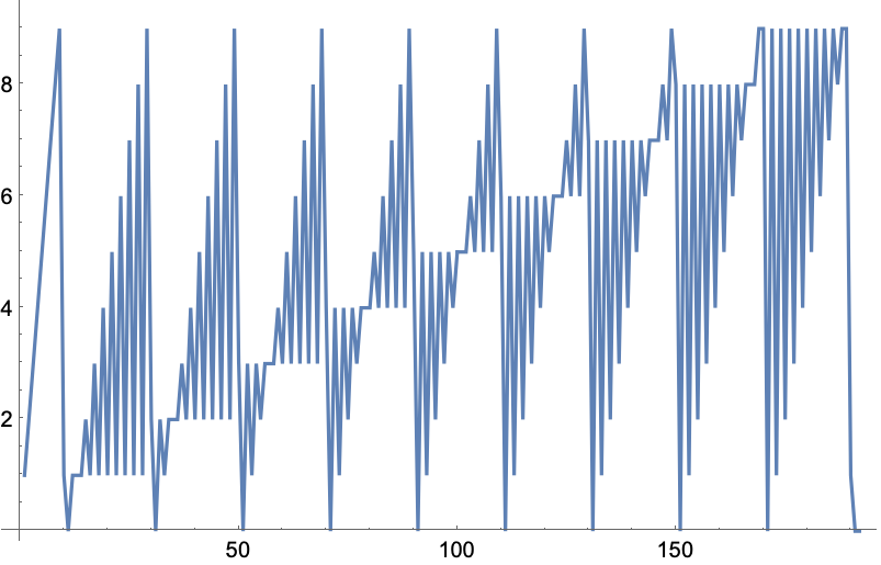
21.5Make a line plot of the result of concatenating all digits of all integers from 1 to 100 (i.e. ..., 8, 9, 1, 0, 1, 1, 1, 2, ...). »
21.8Make a graph in which each connection connects i to j-i, where i and j both range from 1 to 5. »
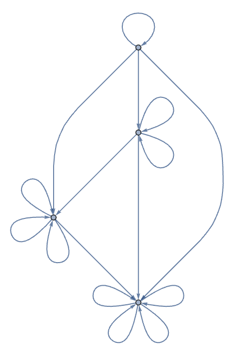
21.9Generate a graph with 100 nodes, each with a connection going to one randomly chosen node. »
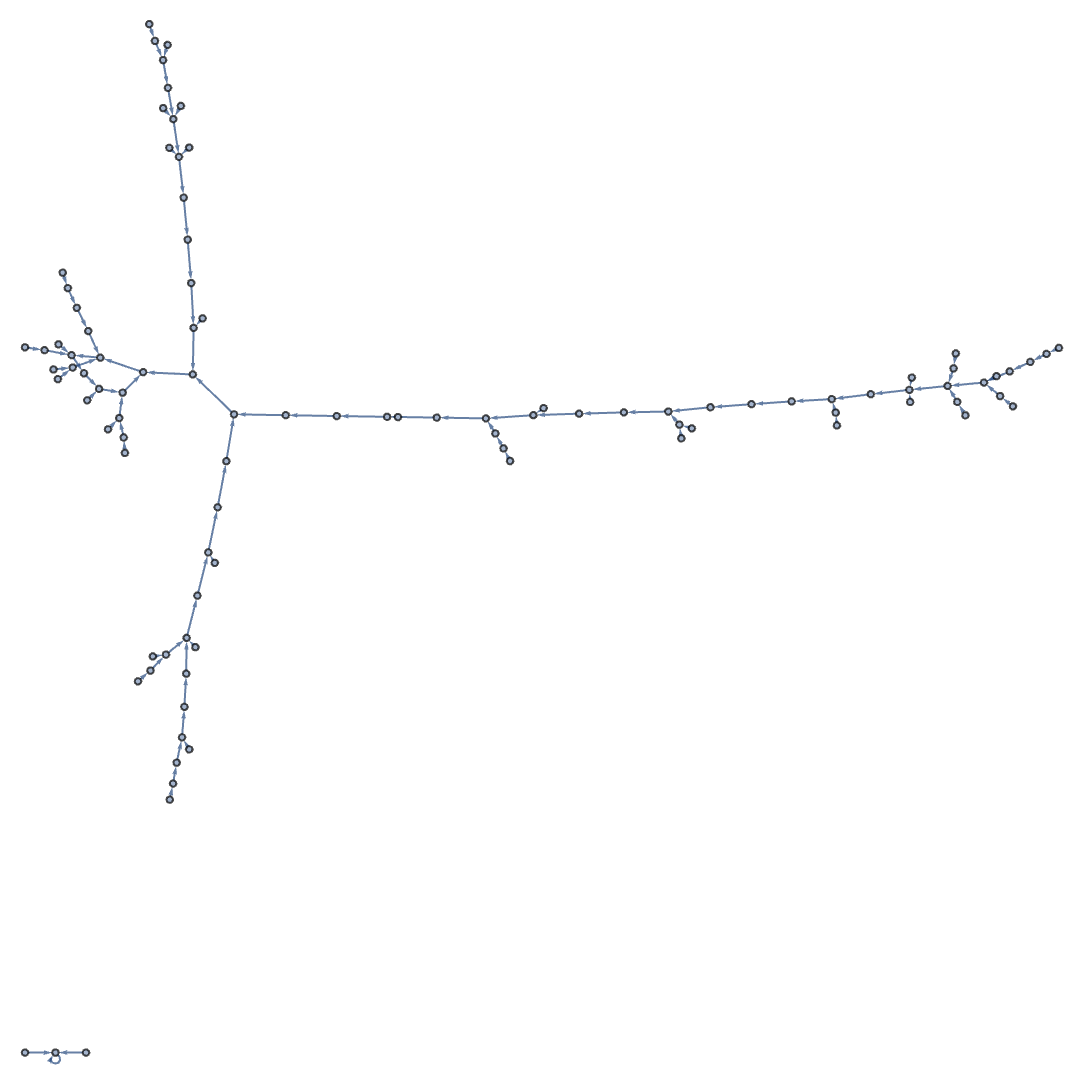
21.10Generate a graph with 100 nodes, each connecting to two randomly chosen nodes. »
21.11For the graph {12, 23, 34, 41, 31, 22}, make a grid giving the shortest paths between every pair of nodes, with the start node as row and end node as column. »

+21.1Make a graph with 4 nodes in which every node is connected, displaying the resulting graph with radial drawing. »
+21.2Generate a graph in which a single node is connected to 10 others. »
+21.3Use Flatten to generate a table of the numbers 1 to 50 in which even numbers are colored red. »
+21.4Use ImageData, Flatten and Total to find the number of white pixels in Binarize[Rasterize["W"]]. »
+21.5Use Flatten, IntegerDigits and Total to find the sum of all digits of all whole numbers up to 1000. »
+21.6Generate a graph with 200 connections, each between nodes with numbers randomly chosen between 0 and 100. »
+21.7Generate a plot that shows communities in a random graph with nodes numbered between 0 and 100, and 200 connections. »
What’s the difference between a “graph” and a “network”?
There’s no difference. They’re just different words for the same thing, though “graph” tends to be more common in math and other formal areas, and “network” more common in more applied areas.
What are the vertices and edges of a graph?
Vertices are the points, or nodes, of a graph. Edges are the connections. Because graphs have arisen in so many different places, there are quite a few different names used for the same thing.
How is ij understood?
It’s Rule[i, j]. Rules are used in lots of places in the Wolfram Language—such as giving settings for options.
How does the Wolfram Language determine how to lay out graphs?
It uses a variety of methods to try to make them as “untangled” and “balanced” as possible. One method is essentially a mechanical simulation in which each edge is like a spring that tries to get shorter, and every node “electrically repels” others. The option GraphLayout lets you specify a layout method to use.
How big a graph can the Wolfram Language handle?
It’s mostly limited by the amount of memory in your computer. Graphs with tens or hundreds of thousands of nodes are not a problem.
Can I specify annotations to nodes and edges?
Yes. You can give Graph lists of nodes and edges that include things like Annotation[node, VertexStyleRed] or Annotation[edge, EdgeWeight20]. You can extract these annotations using AnnotationValue. You can also give overall options to Graph. In addition, you can specify “tags” for edges using, for example, DirectedEdge[i, j, tag]. Tags are displayed if you use EdgeLabelsAutomatic.
- Graphs, like strings, images, graphics, etc., are first-class objects in the Wolfram Language.
- You can enter undirected edges in a graph using <->, which displays as .
- CompleteGraph[n] gives the completely connected graph with n nodes. Among other kinds of special graphs are GridGraph, TorusGraph, KaryTree, etc.
- There are lots of ways to make random graphs (random connections, random numbers of connections, scale-free networks, etc.). RandomGraph[{100, 200}] makes a random graph with 100 nodes and 200 edges.
- AdjacencyMatrix[graph] gives the adjacency matrix for a graph. AdjacencyGraph[matrix] constructs a graph from an adjacency matrix.
- Common settings for the GraphLayout option are "SpringElectricalEmbedding" and "LayeredDigraphEmbedding".
- PlanarGraph[graph] tries to lay a graph out without any edges crossing—if that’s possible.