There’s a lot more to the Wolfram Language than we’ve been able to cover in this book. Here’s a sampling of just a few of the many topics and areas that we’ve missed.
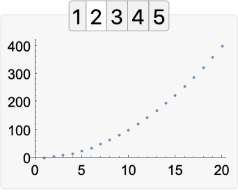
User Interface Construction
Set up a tabbed interface:
In[1]:=
Out[1]=
User interfaces are just another type of symbolic expression; make a grid of sliders:
In[2]:=
Out[2]=

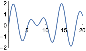
Function Visualization
Plot a function:
In[3]:=
Out[3]=
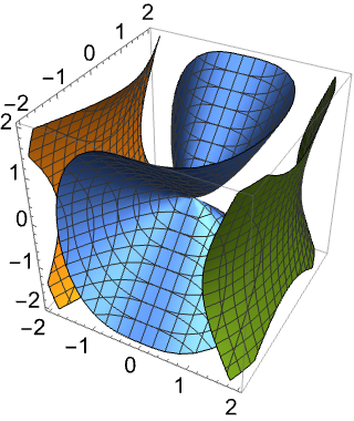
3D contour plot:
In[4]:=
Out[4]=
Mathematical Computation
Do symbolic computations, with x as an algebraic variable:
In[5]:=
Out[5]=
Get symbolic solutions to equations:
In[6]:=
Out[6]=
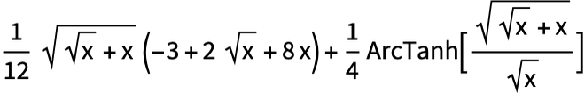
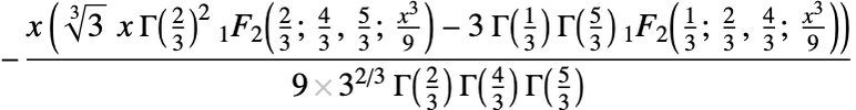
Do calculus symbolically:
In[7]:=
Out[7]=
Display results in traditional mathematical form:
In[8]:=
Out[8]=
Use 2D notation for input:
In[9]:=
Out[9]=
Numerics
Minimize a function inside a spherical ball:
In[10]:=
Out[10]=
In[11]:=
Out[11]=
Make a plot using the approximate function:
In[12]:=
Out[12]=

Geometry
The area of a disk (filled circle) of radius r:
In[13]:=
Out[13]=
Find a circle going through three points:
In[14]:=
Out[14]=
Make a shape by “shrinkwrapping” around 100 random points in 3D:
In[15]:=
Out[15]=

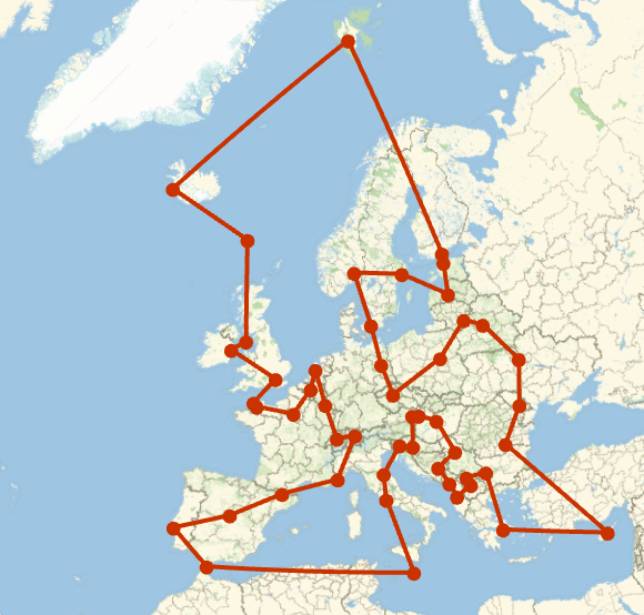
Algorithms
Find the shortest tour of the capitals of Europe (traveling salesman problem):
In[16]:=
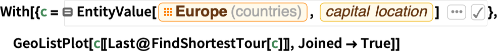
Out[16]=
Factor a big number:
In[17]:=
Out[17]=
Logic
Make a truth table:
In[18]:=
Out[18]=
Find a minimal representation of a Boolean function:
In[19]:=
Out[19]=
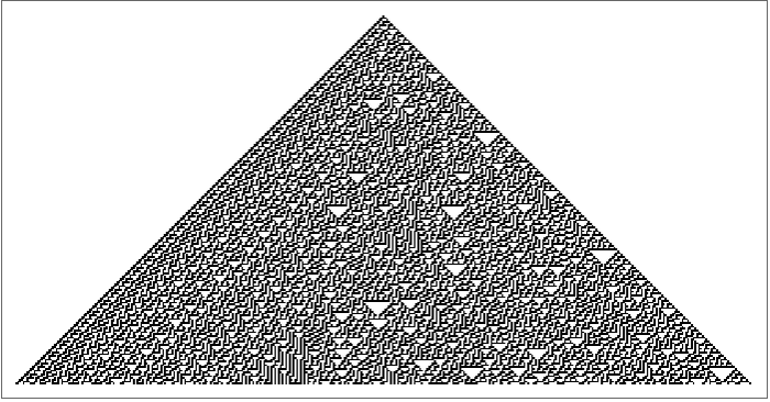
The Computational Universe
Run my favorite example of a very simple program with very complex behavior:
In[20]:=
Out[20]=
RulePlot shows the underlying rule:
In[21]:=
Out[21]=
Chemical & Biological Computation
Enter a specification of a molecule:
In[22]:=
Out[22]=
Make a 3D representation of the molecule:
In[23]:=
Out[23]=
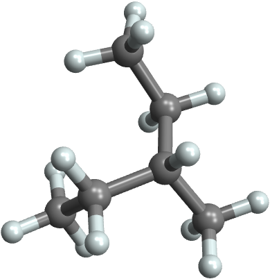
In[24]:=
Out[24]=
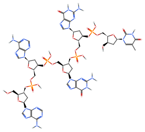
Draw the corresponding molecule:
In[25]:=
Out[25]=
Building APIs
Deploy a simple web API that finds the distance from a specified location:
In[26]:=
Out[26]=
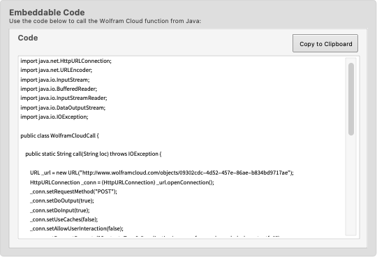
Create embeddable code for an external Java program to call the API:
In[27]:=
Out[27]=
Document Generation
Documents are symbolic expressions, like everything else:
In[28]:=
Out[28]=

Evaluation Control
Hold a computation unevaluated:
In[29]:=
Out[29]=
Release the hold:
In[30]:=
Out[30]=
Systems-Level Operations
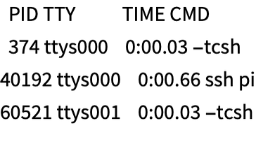
Run an external process (not allowed in the cloud!):
In[31]:=
Out[31]=
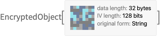
Encrypt anything:
In[32]:=
Out[32]=
Parallel Computation
I’m running on a 28-core machine:
In[33]:=
Out[33]=
Sequentially test a sequence of (big) numbers for primality, and find the total time taken:
In[34]:=
Out[34]=
Doing the same thing in parallel takes considerably less time:
In[35]:=
Out[35]=