Model Small Oscillations in a CO Molecule
Experimentally, a CO molecule oscillates about its equilibrium length with an effective spring constant of  . The oscillations are governed by the quantum harmonic oscillator equation. In the following,
  is the reduced mass of the molecule,
  is the natural frequency,
  is the displacement from the equilibrium position, and
  is the reduced Planck's constant.
qho = -(\[HBar]^2/(2 m)) Laplacian[u[x], {x}] + (m \[Omega]^2)/
2 x^2 u[x];Compute the first four eigenvalues and normalized eigenfunctions.
sol = DEigensystem[qho, u[x], {x, -\[Infinity], \[Infinity]}, 4,
  Assumptions -> \[HBar] > 0 && m > 0 && \[Omega] > 0,
  Method -> "Normalize"]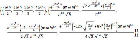
Assuming the particle is in an equal superposition of the four states, the wavefunction will have the form  .
.
\[Psi][x_, t_] = Total[MapThread[1/2 Exp[I E t #1/\[HBar]] #2 &, sol]]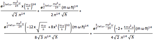
Compute the three parameters  ,
,  , and
, and  using base units of atomic mass units, femtoseconds, and picometers, as the resulting values will be close to order unity.
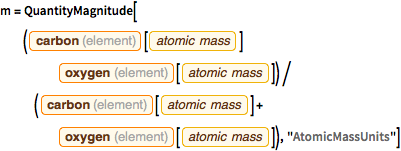
m = QuantityMagnitude[(
  Entity["Element", "Carbon"][
    EntityProperty["Element", "AtomicMass"]] Entity["Element",
     "Oxygen"][EntityProperty["Element", "AtomicMass"]])/(
  Entity["Element", "Carbon"][
    EntityProperty["Element", "AtomicMass"]] +
   Entity["Element", "Oxygen"][
    EntityProperty["Element", "AtomicMass"]]), "AtomicMassUnits"]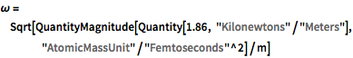
\[Omega] =
 Sqrt[QuantityMagnitude[Quantity[1.86, "Kilonewtons"/"Meters"],
"AtomicMassUnit"/"Femtoseconds"^2]/m]\[HBar] =
QuantityMagnitude[Quantity[1., "ReducedPlanckConstant"],
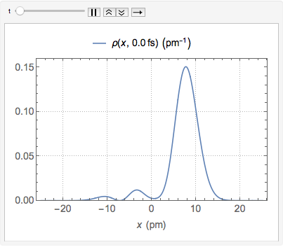
"AtomicMassUnit"*"Picometers"^2/"Femtoseconds"]The probability density function of the displacement is given by  .
.
\[Rho][x_, t_] =
 FullSimplify[ComplexExpand[Conjugate[\[Psi][x, t]] \[Psi][x, t]]]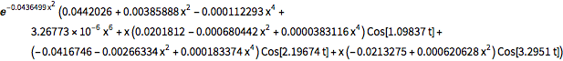
As a probability distribution, the integral of  over the reals is 1 for all
  .
.
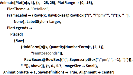
Chop[Integrate[\[Rho][x, t], {x, -\[Infinity], \[Infinity]}]]Visualize the probability density over time.