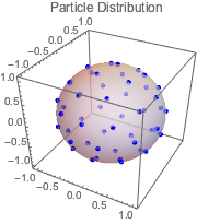
球体上の電荷分布を求める
球体上を自由に移動する等電荷粒子のクーロン(Coulomb)ポテンシャルを最小化する位置を求める.これは平衡電荷分布である.
粒子の数を n で表す.
In[1]:=
n = 50; を
を 
![]() 番目の粒子の直交座標とする.
番目の粒子の直交座標とする.
In[2]:=
vars = Join[Array[x, n], Array[y, n], Array[z, n]];目標は,クーロンポテンシャルを最小化することである.
In[3]:=
potential =
  Sum[((x[i] - x[j])^2 + (y[i] - y[j])^2 + (z[i] - z[j])^2)^-(1/
       2), {i, 1, n - 1}, {j, i + 1, n}];
粒子は球体上にあるので,それらの座標は1という制約条件を満足しなければならない.
In[4]:=
sphereconstr = Table[x[i]^2 + y[i]^2 + z[i]^2 == 1, {i, 1, n}];球座標を使って,球体上の初期点をランダムに選ぶ.
In[5]:=
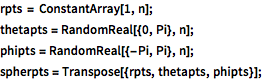
rpts = ConstantArray[1, n];
thetapts = RandomReal[{0, Pi}, n];
phipts = RandomReal[{-Pi, Pi}, n];
spherpts = Transpose[{rpts, thetapts, phipts}];
初期点を直交座標に変換する.
In[6]:=
cartpts = CoordinateTransform["Spherical" -> "Cartesian", spherpts];変数の順にマッチするよう,初期点を並べ替える.
In[7]:=
initpts = Flatten[Transpose[cartpts]];球の制約条件の対象となるクーロンポテンシャルを最小化する.
In[8]:=
sol = FindMinimum[{potential, sphereconstr}, Thread[{vars, initpts}]];粒子の平衡位置を解から取り出す.
In[9]:=
solpts = Table[{x[i], y[i], z[i]}, {i, 1, n}] /. sol[[2]];結果をプロットする.
In[10]:=
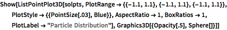
Show[ListPointPlot3D[solpts,
  PlotRange -> {{-1.1, 1.1}, {-1.1, 1.1}, {-1.1, 1.1}},
  PlotStyle -> {{PointSize[.03], Blue}}, AspectRatio -> 1,
  BoxRatios -> 1, PlotLabel -> "Particle Distribution"],
 Graphics3D[{Opacity[.5], Sphere[]}]]
Out[10]=