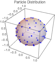
求球面上的电荷分布: Wolfram语言 11 的新功能

‹›

求球面上的电荷分布

找出球面上使库仑势为最小的自由运动等电荷粒子的位置，这便是平衡时的电荷分布.

用 n 表示粒子数.

In[1]:=

n = 50;

设 {x_i, y_i, z_i} 为粒子的笛卡尔坐标.

In[2]:=

vars = Join[Array[x, n], Array[y, n], Array[z, n]];

目标是使库仑势最小.

In[3]:=

potential = 
  Sum[((x[i] - x[j])^2 + (y[i] - y[j])^2 + (z[i] - z[j])^2)^-(1/
       2), {i, 1, n - 1}, {j, i + 1, n}];

由于粒子是在球面上，它们的坐标必须满足大小为 1 的约束.

In[4]:=

sphereconstr = Table[x[i]^2 + y[i]^2 + z[i]^2 == 1, {i, 1, n}];

使用球面坐标在球面上随机选择初始点.

In[5]:=

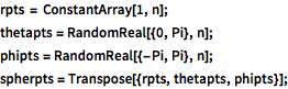
rpts = ConstantArray[1, n];
thetapts = RandomReal[{0, Pi}, n];
phipts = RandomReal[{-Pi, Pi}, n];
spherpts = Transpose[{rpts, thetapts, phipts}];

将初始点变换成笛卡尔坐标.

In[6]:=

cartpts = CoordinateTransform["Spherical" -> "Cartesian", spherpts];

重新排列初始点使其与变量顺序匹配.

In[7]:=

initpts = Flatten[Transpose[cartpts]];

以球面为约束将库仑势最小化.

In[8]:=

sol = FindMinimum[{potential, sphereconstr}, Thread[{vars, initpts}]];

从解当中提取出粒子的平衡位置.

In[9]:=

solpts = Table[{x[i], y[i], z[i]}, {i, 1, n}] /. sol[[2]];

图示结果.

In[10]:=

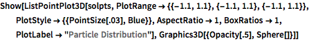
Show[ListPointPlot3D[solpts, 
  PlotRange -> {{-1.1, 1.1}, {-1.1, 1.1}, {-1.1, 1.1}}, 
  PlotStyle -> {{PointSize[.03], Blue}}, AspectRatio -> 1, 
  BoxRatios -> 1, PlotLabel -> "Particle Distribution"], 
 Graphics3D[{Opacity[.5], Sphere[]}]]

Out[10]=

Wolfram 语言™

求球面上的电荷分布

相关范例