Wolfram 语言™

矩阵正态和矩阵 T 分布

Matrix 正态和矩阵 分布是具有指定行和列尺度矩阵的矩阵变元正态和 分布. 典型用途包括时间序列分析、随机过程和多元回归等.

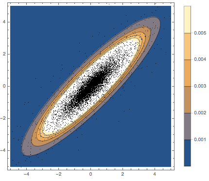
已知尺度矩阵 Σ_row 和 Σ_col，矩阵正态分布的概率密度与 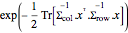成比例. 以下是来自一个矩阵正态分布的样本.

In[1]:=

Subscript[\[CapitalSigma], row] = {{1, 0.9}, {0.9, 1}}; Subscript[\[CapitalSigma], col] = {{1, -0.9}, {-0.9, 1}};

In[2]:=

RandomVariate[ MatrixNormalDistribution[Subscript[\[CapitalSigma], row], Subscript[\[CapitalSigma], col]]]

Out[2]=

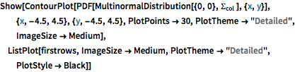
在散点图上可视化行向量样本，并与密度函数比较.

In[3]:=

sample = RandomVariate[ MatrixNormalDistribution[Subscript[\[CapitalSigma], row], Subscript[\[CapitalSigma], col]], 10^4]; firstrows = sample[[All, 1]];

In[4]:=

Show[ContourPlot[ PDF[MultinormalDistribution[{0, 0}, Subscript[\[CapitalSigma], col] ], {x, y}], {x, -4.5, 4.5}, {y, -4.5, 4.5}, PlotPoints -> 30, PlotTheme -> "Detailed", ImageSize -> Medium], ListPlot[firstrows, ImageSize -> Medium, PlotTheme -> "Detailed", PlotStyle -> Black]]

Out[4]=

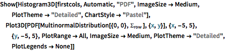
在直方图上可视化列向量样本，并与密度函数比较.

In[5]:=

firstcols = sample[[All, All, 1]];

In[6]:=

Show[Histogram3D[firstcols, Automatic, "PDF", ImageSize -> Medium, PlotTheme -> "Detailed", ChartStyle -> "Pastel"], Plot3D[PDF[ MultinormalDistribution[{0, 0}, Subscript[\[CapitalSigma], row] ], {x, y}], {x, -5, 5}, {y, -5, 5}, PlotRange -> All, ImageSize -> Medium, PlotTheme -> "Detailed", PlotLegends -> None]]

Out[6]=

与学生 和多变元 分布相似，矩阵 分布是矩阵正态分布与逆 Wishart 分布的尺度参数的混合. 以下是来自矩阵 分布的样本.

In[7]:=

RandomVariate[ MatrixTDistribution[Subscript[\[CapitalSigma], row], Subscript[\[CapitalSigma], col], 3]]

Out[7]=

生成一组矩阵 分布的矩阵.

In[8]:=

sample = RandomVariate[ MatrixTDistribution[Subscript[\[CapitalSigma], row], Subscript[\[CapitalSigma], col], 3], 10^4];

矩阵 分布的变元的低维投影是学生 和多变元 分布. 将样本投影到二维向量上，并验证拟合优度.

In[9]:=

v = {1, 2}; vecs = sample.v;

In[10]:=

DistributionFitTest[vecs, MultivariateTDistribution[ Subscript[\[CapitalSigma], row] (v.Subscript[\[CapitalSigma], col].v)/3, 3]]

Out[10]=

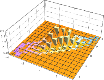
在散点图上可视化投影数据，并将其与密度函数比较.

In[11]:=

Show[ContourPlot[ PDF[MultivariateTDistribution[ Subscript[\[CapitalSigma], row] (v.Subscript[\[CapitalSigma], col].v)/3, 3], {x, y}], {x, -5, 5}, {y, -5, 5}, PlotPoints -> 30, PlotTheme -> "Detailed", ImageSize -> Medium], ListPlot[vecs, ImageSize -> Medium, PlotTheme -> "Detailed", PlotStyle -> Black]]

Out[11]=