Modélisez une chaîne pendante

Trouvez la position avec l'énergie potentielle minimale d'une chaîne ou d'un fil de longueur suspendue entre deux points.

Configurez les valeurs de paramètre de la longueur de la chaîne , la hauteur de l'extrémité gauche et la hauteur de l'extrémité droite .

In[1]:=

L = 4; a = 1; b = 3;

Soit , la hauteur de la chaîne comme fonction de position horizontale, avec .

In[2]:=

xf = 1; nh = 201; h := xf/nh;

Configurez les variables pour la hauteur de la chaîne .

In[3]:=

varsy = Array[y, nh + 1, {0, nh}];

Désignez la pente à la position par et configurez-lui des variables.

In[4]:=

varsm = Array[m, nh + 1, {0, nh}];

Désignez l'énergie potentielle partielle de à par .

In[5]:=

varsv = Array[v, nh + 1, {0, nh}];

Désignez la longueur de la chaîne à la position par et configurez-lui des variables.

In[6]:=

varss = Array[s, nh + 1, {0, nh}];

Joignez toutes les variables.

In[7]:=

vars = Join[varsm, varsy, varsv, varss];

L'objectif est de minimiser l'énergie potentielle totale .

In[8]:=

objfn = v[nh];

Voici la valeur limite des contraintes géométriques.

In[9]:=

bndcons = {y[0] == a, y[nh] == b, v[0] == 0, s[0] == 0, s[nh] == L};

Discrétisez les EDO : , , .

In[10]:=

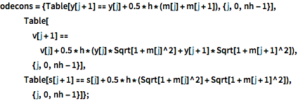
odecons = {Table[ y[j + 1] == y[j] + 0.5*h*(m[j] + m[j + 1]), {j, 0, nh - 1}], Table[v[j + 1] == v[j] + 0.5* h*(y[j]*Sqrt[1 + m[j]^2] + y[j + 1]*Sqrt[1 + m[j + 1]^2]), {j, 0, nh - 1}], Table[s[j + 1] == s[j] + 0.5*h*(Sqrt[1 + m[j]^2] + Sqrt[1 + m[j + 1]^2]), {j, 0, nh - 1}]};

Choisissez des points initiaux pour les variables.

In[11]:=

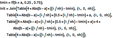
tmin = If[b > a, 0.25 , 0.75]; init = Join[Table[4*Abs[b - a]*((k/nh) - tmin), {k, 0, nh}], Table[4*Abs[b - a]*(k/nh)*(0.5*(k/nh) - tmin) + a, {k, 0, nh}], Table[(4*Abs[b - a]*(k/nh)*(0.5*(k/nh) - tmin) + a)*4* Abs[b - a]*((k/nh) - tmin), {k, 0, nh}], Table[4*Abs[b - a]*((k/nh) - tmin), {k, 0, nh}]];

Minimisez l'énergie potentielle totale, sous réserve des contraintes.

In[12]:=

sol = FindMinimum[{objfn, Join[bndcons, odecons]}, Thread[{vars, init}]];

Extrayez les points de solution.

In[13]:=

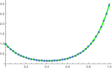
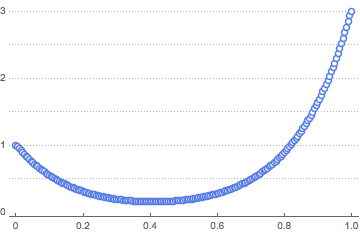
solpts = Table[{i h, y[i] /. sol[[2]]}, {i, 0, nh}];

Tracez la position de la chaîne avec un minimum d'énergie potentielle.

In[14]:=

ListPlot[solpts, ImageSize -> Medium, PlotTheme -> "Marketing"]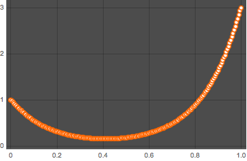

Out[14]=

Utilisez FindFit pour adapter le résultat à la courbe caténaire.

In[15]:=

catenary[t_] = c1 + (1/c2) Cosh[c2 (t - c3)];

In[16]:=

fitsol = FindFit[solpts, catenary[t], {c1, c2, c3}, {t}]

Out[16]=

Tracez les points de solution avec la courbe caténaire.

In[17]:=

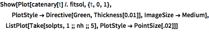
Show[Plot[catenary[t] /. fitsol, {t, 0, 1}, PlotStyle -> Directive[Green, Thickness[0.01]], ImageSize -> Medium], ListPlot[Take[solpts, 1 ;; nh ;; 5], PlotStyle -> PointSize[.02]]]

Out[17]=